
Go Green With Knowledge! Get 30% off on Annual Courses For World Environment Day with code NATURE30

Share this article

Table of Contents
Latest updates.

Ways To Improve Learning Outcomes: Learn Tips & Tricks
The Three States of Matter: Solids, Liquids, and Gases
Types of Motion: Introduction, Parameters, Examples
Understanding Frequency Polygon: Detailed Explanation
Uses of Silica Gel in Packaging?
Visual Learning Style for Students: Pros and Cons
Air Pollution: Know the Causes, Effects & More
Sexual Reproduction in Flowering Plants
Integers Introduction: Check Detailed Explanation
Human Respiratory System – Detailed Explanation
Tag cloud :.
- entrance exams
- engineering
- ssc cgl 2024
- Written By Priya_Singh
- Last Modified 24-01-2023
Data Representation: Definition, Types, Examples
Data Representation: Data representation is a technique for analysing numerical data. The relationship between facts, ideas, information, and concepts is depicted in a diagram via data representation. It is a fundamental learning strategy that is simple and easy to understand. It is always determined by the data type in a specific domain. Graphical representations are available in many different shapes and sizes.
In mathematics, a graph is a chart in which statistical data is represented by curves or lines drawn across the coordinate point indicated on its surface. It aids in the investigation of a relationship between two variables by allowing one to evaluate the change in one variable’s amount in relation to another over time. It is useful for analysing series and frequency distributions in a given context. On this page, we will go through two different types of graphs that can be used to graphically display data. Continue reading to learn more.

Data Representation in Maths
Definition: After collecting the data, the investigator has to condense them in tabular form to study their salient features. Such an arrangement is known as the presentation of data.
Any information gathered may be organised in a frequency distribution table, and then shown using pictographs or bar graphs. A bar graph is a representation of numbers made up of equally wide bars whose lengths are determined by the frequency and scale you choose.
The collected raw data can be placed in any one of the given ways:
- Serial order of alphabetical order
- Ascending order
- Descending order
Data Representation Example
Example: Let the marks obtained by \(30\) students of class VIII in a class test, out of \(50\)according to their roll numbers, be:
\(39,\,25,\,5,\,33,\,19,\,21,\,12,41,\,12,\,21,\,19,\,1,\,10,\,8,\,12\)
\(17,\,19,\,17,\,17,\,41,\,40,\,12,41,\,33,\,19,\,21,\,33,\,5,\,1,\,21\)
The data in the given form is known as raw data or ungrouped data. The above-given data can be placed in the serial order as shown below:

Now, for say you want to analyse the standard of achievement of the students. If you arrange them in ascending or descending order, it will give you a better picture.
Ascending order:
\(1,\,1,\,5,\,5,\,8,\,10,\,12,12,\,12,\,12,\,17,\,17,\,17,\,19,\,19\)
\(19,\,19,\,21,\,21,\,21,\,25,\,33,33,\,33,\,39,\,40,\,41,\,41,\,41\)
Descending order:
\(41,\,41,\,41,\,40,\,39,\,33,\,33,33,\,25,\,21,\,21,\,21,\,21,\,19,\,19\)
\(19,\,19,\,17,\,17,\,17,\,12,\,12,12,\,12,\,10,\,8,\,5,\,5,1,\,1\)
When the raw data is placed in ascending or descending order of the magnitude is known as an array or arrayed data.
Graph Representation in Data Structure
A few of the graphical representation of data is given below:
- Frequency distribution table
Pictorial Representation of Data: Bar Chart
The bar graph represents the qualitative data visually. The information is displayed horizontally or vertically and compares items like amounts, characteristics, times, and frequency.
The bars are arranged in order of frequency, so more critical categories are emphasised. By looking at all the bars, it is easy to tell which types in a set of data dominate the others. Bar graphs can be in many ways like single, stacked, or grouped.

Graphical Representation of Data: Frequency Distribution Table
A frequency table or frequency distribution is a method to present raw data in which one can easily understand the information contained in the raw data.
The frequency distribution table is constructed by using the tally marks. Tally marks are a form of a numerical system with the vertical lines used for counting. The cross line is placed over the four lines to get a total of \(5\).

Consider a jar containing the different colours of pieces of bread as shown below:

Construct a frequency distribution table for the data mentioned above.

Graphical Representation of Data: Histogram
The histogram is another kind of graph that uses bars in its display. The histogram is used for quantitative data, and ranges of values known as classes are listed at the bottom, and the types with greater frequencies have the taller bars.
A histogram and the bar graph look very similar; however, they are different because of the data level. Bar graphs measure the frequency of the categorical data. A categorical variable has two or more categories, such as gender or hair colour.

Graphical Representation of Data: Pie Chart
The pie chart is used to represent the numerical proportions of a dataset. This graph involves dividing a circle into different sectors, where each of the sectors represents the proportion of a particular element as a whole. Thus, it is also known as a circle chart or circle graph.

Graphical Representation of Data: Line Graph
A graph that uses points and lines to represent change over time is defined as a line graph. In other words, it is the chart that shows a line joining multiple points or a line that shows the link between the points.
The diagram illustrates the quantitative data between two changing variables with the straight line or the curve that joins a series of successive data points. Linear charts compare two variables on the vertical and the horizontal axis.

General Rules for Visual Representation of Data
We have a few rules to present the information in the graphical representation effectively, and they are given below:
- Suitable Title: Ensure that the appropriate title is given to the graph, indicating the presentation’s subject.
- Measurement Unit: Introduce the measurement unit in the graph.
- Proper Scale: To represent the data accurately, choose an appropriate scale.
- Index: In the Index, the appropriate colours, shades, lines, design in the graphs are given for better understanding.
- Data Sources: At the bottom of the graph, include the source of information wherever necessary.
- Keep it Simple: Build the graph in a way that everyone should understand easily.
- Neat: You have to choose the correct size, fonts, colours etc., in such a way that the graph must be a model for the presentation of the information.
Solved Examples on Data Representation
Q.1. Construct the frequency distribution table for the data on heights in \(({\rm{cm}})\) of \(20\) boys using the class intervals \(130 – 135,135 – 140\) and so on. The heights of the boys in \({\rm{cm}}\) are:

Ans: The frequency distribution for the above data can be constructed as follows:

Q.2. Write the steps of the construction of Bar graph? Ans: To construct the bar graph, follow the given steps: 1. Take a graph paper, draw two lines perpendicular to each other, and call them horizontal and vertical. 2. You have to mark the information given in the data like days, weeks, months, years, places, etc., at uniform gaps along the horizontal axis. 3. Then you have to choose the suitable scale to decide the heights of the rectangles or the bars and then mark the sizes on the vertical axis. 4. Draw the bars or rectangles of equal width and height marked in the previous step on the horizontal axis with equal spacing. The figure so obtained will be the bar graph representing the given numerical data.
Q.3. Read the bar graph and then answer the given questions: I. Write the information provided by the given bar graph. II. What is the order of change of the number of students over several years? III. In which year is the increase of the student maximum? IV. State whether true or false. The enrolment during \(1996 – 97\) is double that of \(1995 – 96\)

Ans: I. The bar graph represents the number of students in class \({\rm{VI}}\) of a school during the academic years \(1995 – 96\,to\,1999 – 2000\). II. The number of stcccccudents is changing in increasing order as the heights of bars are growing. III. The increase in the number of students in uniform and the increase in the height of bars is uniform. Hence, in this case, the growth is not maximum in any of the years. The enrolment in the years is \(1996 – 97\, = 200\). and the enrolment in the years is \(1995 – 96\, = 150\). IV. The enrolment in \(1995 – 97\,\) is not double the enrolment in \(1995 – 96\). So the statement is false.
Q.4. Write the frequency distribution for the given information of ages of \(25\) students of class VIII in a school. \(15,\,16,\,16,\,14,\,17,\,17,\,16,\,15,\,15,\,16,\,16,\,17,\,15\) \(16,\,16,\,14,\,16,\,15,\,14,\,15,\,16,\,16,\,15,\,14,\,15\) Ans: Frequency distribution of ages of \(25\) students:

Q.5. There are \(20\) students in a classroom. The teacher asked the students to talk about their favourite subjects. The results are listed below:

By looking at the above data, which is the most liked subject? Ans: Representing the above data in the frequency distribution table by using tally marks as follows:

From the above table, we can see that the maximum number of students \((7)\) likes mathematics.
Also, Check –
- Diagrammatic Representation of Data
In the given article, we have discussed the data representation with an example. Then we have talked about graphical representation like a bar graph, frequency table, pie chart, etc. later discussed the general rules for graphic representation. Finally, you can find solved examples along with a few FAQs. These will help you gain further clarity on this topic.

FAQs on Data Representation
Q.1: How is data represented? A: The collected data can be expressed in various ways like bar graphs, pictographs, frequency tables, line graphs, pie charts and many more. It depends on the purpose of the data, and accordingly, the type of graph can be chosen.
Q.2: What are the different types of data representation? A : The few types of data representation are given below: 1. Frequency distribution table 2. Bar graph 3. Histogram 4. Line graph 5. Pie chart
Q.3: What is data representation, and why is it essential? A: After collecting the data, the investigator has to condense them in tabular form to study their salient features. Such an arrangement is known as the presentation of data. Importance: The data visualization gives us a clear understanding of what the information means by displaying it visually through maps or graphs. The data is more natural to the mind to comprehend and make it easier to rectify the trends outliners or trends within the large data sets.
Q.4: What is the difference between data and representation? A: The term data defines the collection of specific quantitative facts in their nature like the height, number of children etc., whereas the information in the form of data after being processed, arranged and then presented in the state which gives meaning to the data is data representation.
Q.5: Why do we use data representation? A: The data visualization gives us a clear understanding of what the information means by displaying it visually through maps or graphs. The data is more natural to the mind to comprehend and make it easier to rectify the trends outliners or trends within the large data sets.
Related Articles
Ways To Improve Learning Outcomes: With the development of technology, students may now rely on strategies to enhance learning outcomes. No matter how knowledgeable a...
The Three States of Matter: Anything with mass and occupied space is called ‘Matter’. Matters of different kinds surround us. There are some we can...
Motion is the change of a body's position or orientation over time. The motion of humans and animals illustrates how everything in the cosmos is...
Understanding Frequency Polygon: Students who are struggling with understanding Frequency Polygon can check out the details here. A graphical representation of data distribution helps understand...
When you receive your order of clothes or leather shoes or silver jewellery from any online shoppe, you must have noticed a small packet containing...
Visual Learning Style: We as humans possess the power to remember those which we have caught visually in our memory and that too for a...
Air Pollution: In the past, the air we inhaled was pure and clean. But as industrialisation grows and the number of harmful chemicals in the...
In biology, flowering plants are known by the name angiosperms. Male and female reproductive organs can be found in the same plant in flowering plants....
Integers Introduction: To score well in the exam, students must check out the Integers introduction and understand them thoroughly. The collection of negative numbers and whole...
Human Respiratory System: Students preparing for the NEET and Biology-related exams must have an idea about the human respiratory system. It is a network of tissues...
Place Value of Numbers: Detailed Explanation
Place Value of Numbers: Students must understand the concept of the place value of numbers to score high in the exam. In mathematics, place value...
The Leaf: Types, Structures, Parts
The Leaf: Students who want to understand everything about the leaf can check out the detailed explanation provided by Embibe experts. Plants have a crucial role...
Factors Affecting Respiration: Definition, Diagrams with Examples
In plants, respiration can be regarded as the reversal of the photosynthetic process. Like photosynthesis, respiration involves gas exchange with the environment. Unlike photosynthesis, respiration...
General Terms Related to Spherical Mirrors
General terms related to spherical mirrors: A mirror with the shape of a portion cut out of a spherical surface or substance is known as a...
Number System: Types, Conversion and Properties
Number System: Numbers are highly significant and play an essential role in Mathematics that will come up in further classes. In lower grades, we learned how...
Types of Respiration
Every living organism has to "breathe" to survive. The process by which the living organisms use their food to get energy is called respiration. It...
Animal Cell: Definition, Diagram, Types of Animal Cells
Animal Cell: An animal cell is a eukaryotic cell with membrane-bound cell organelles without a cell wall. We all know that the cell is the fundamental...
Conversion of Percentages: Conversion Method & Examples
Conversion of Percentages: To differentiate and explain the size of quantities, the terms fractions and percent are used interchangeably. Some may find it difficult to...
Arc of a Circle: Definition, Properties, and Examples
Arc of a circle: A circle is the set of all points in the plane that are a fixed distance called the radius from a fixed point...
Ammonia (NH3): Preparation, Structure, Properties and Uses
Ammonia, a colourless gas with a distinct odour, is a chemical building block and a significant component in producing many everyday items. It is found...
CGPA to Percentage: Calculator for Conversion, Formula, & More
CGPA to Percentage: The average grade point of a student is calculated using their cumulative grades across all subjects, omitting any supplemental coursework. Many colleges,...
Uses of Ether – Properties, Nomenclature, Uses, Disadvantages
Uses of Ether: Ether is an organic compound containing an oxygen atom and an ether group connected to two alkyl/aryl groups. It is formed by the...
General and Middle Terms: Definitions, Formula, Independent Term, Examples
General and Middle terms: The binomial theorem helps us find the power of a binomial without going through the tedious multiplication process. Further, the use...
Mutually Exclusive Events: Definition, Formulas, Solved Examples
Mutually Exclusive Events: In the theory of probability, two events are said to be mutually exclusive events if they cannot occur simultaneously or at the...
Geometry: Definition, Shapes, Structure, Examples
Geometry is a branch of mathematics that is largely concerned with the forms and sizes of objects, their relative positions, and the qualities of space....
Bohr’s Model of Hydrogen Atom: Expressions for Radius, Energy
Rutherford’s Atom Model was undoubtedly a breakthrough in atomic studies. However, it was not wholly correct. The great Danish physicist Niels Bohr (1885–1962) made immediate...
Types of Functions: Definition, Classification and Examples
Types of Functions: Functions are the relation of any two sets. A relation describes the cartesian product of two sets. Cartesian products of two sets...

39 Insightful Publications

Embibe Is A Global Innovator

Innovator Of The Year Education Forever
Interpretable And Explainable AI

Revolutionizing Education Forever

Best AI Platform For Education

Enabling Teachers Everywhere

Decoding Performance

Leading AI Powered Learning Solution Provider

Auto Generation Of Tests

Disrupting Education In India

Problem Sequencing Using DKT

Help Students Ace India's Toughest Exams

Best Education AI Platform

Unlocking AI Through Saas

Fixing Student’s Behaviour With Data Analytics

Leveraging Intelligence To Deliver Results

Brave New World Of Applied AI

You Can Score Higher

Harnessing AI In Education

Personalized Ed-tech With AI

Exciting AI Platform, Personalizing Education
Disruptor Award For Maximum Business Impact

Top 20 AI Influencers In India

Proud Owner Of 9 Patents

Innovation in AR/VR/MR

Best Animated Frames Award 2024
Trending Searches
Previous year question papers, sample papers.
Unleash Your True Potential With Personalised Learning on EMBIBE

Ace Your Exam With Personalised Learning on EMBIBE
Enter mobile number.
By signing up, you agree to our Privacy Policy and Terms & Conditions

- Data representation
Bytes of memory
- Abstract machine
Unsigned integer representation
Signed integer representation, pointer representation, array representation, compiler layout, array access performance, collection representation.
- Consequences of size and alignment rules
Uninitialized objects
Pointer arithmetic, undefined behavior.
- Computer arithmetic
Arena allocation
This course is about learning how computers work, from the perspective of systems software: what makes programs work fast or slow, and how properties of the machines we program impact the programs we write. We want to communicate ideas, tools, and an experimental approach.
The course divides into six units:
- Assembly & machine programming
- Storage & caching
- Kernel programming
- Process management
- Concurrency
The first unit, data representation , is all about how different forms of data can be represented in terms the computer can understand.
Computer memory is kind of like a Lite Brite.

A Lite Brite is big black backlit pegboard coupled with a supply of colored pegs, in a limited set of colors. You can plug in the pegs to make all kinds of designs. A computer’s memory is like a vast pegboard where each slot holds one of 256 different colors. The colors are numbered 0 through 255, so each slot holds one byte . (A byte is a number between 0 and 255, inclusive.)
A slot of computer memory is identified by its address . On a computer with M bytes of memory, and therefore M slots, you can think of the address as a number between 0 and M −1. My laptop has 16 gibibytes of memory, so M = 16×2 30 = 2 34 = 17,179,869,184 = 0x4'0000'0000 —a very large number!
The problem of data representation is the problem of representing all the concepts we might want to use in programming—integers, fractions, real numbers, sets, pictures, texts, buildings, animal species, relationships—using the limited medium of addresses and bytes.
Powers of ten and powers of two. Digital computers love the number two and all powers of two. The electronics of digital computers are based on the bit , the smallest unit of storage, which a base-two digit: either 0 or 1. More complicated objects are represented by collections of bits. This choice has many scale and error-correction advantages. It also refracts upwards to larger choices, and even into terminology. Memory chips, for example, have capacities based on large powers of two, such as 2 30 bytes. Since 2 10 = 1024 is pretty close to 1,000, 2 20 = 1,048,576 is pretty close to a million, and 2 30 = 1,073,741,824 is pretty close to a billion, it’s common to refer to 2 30 bytes of memory as “a giga byte,” even though that actually means 10 9 = 1,000,000,000 bytes. But for greater precision, there are terms that explicitly signal the use of powers of two. 2 30 is a gibibyte : the “-bi-” component means “binary.”
Virtual memory. Modern computers actually abstract their memory spaces using a technique called virtual memory . The lowest-level kind of address, called a physical address , really does take on values between 0 and M −1. However, even on a 16GiB machine like my laptop, the addresses we see in programs can take on values like 0x7ffe'ea2c'aa67 that are much larger than M −1 = 0x3'ffff'ffff . The addresses used in programs are called virtual addresses . They’re incredibly useful for protection: since different running programs have logically independent address spaces, it’s much less likely that a bug in one program will crash the whole machine. We’ll learn about virtual memory in much more depth in the kernel unit ; the distinction between virtual and physical addresses is not as critical for data representation.
Most programming languages prevent their users from directly accessing memory. But not C and C++! These languages let you access any byte of memory with a valid address. This is powerful; it is also very dangerous. But it lets us get a hands-on view of how computers really work.
C++ programs accomplish their work by constructing, examining, and modifying objects . An object is a region of data storage that contains a value, such as the integer 12. (The standard specifically says “a region of data storage in the execution environment, the contents of which can represent values”.) Memory is called “memory” because it remembers object values.
In this unit, we often use functions called hexdump to examine memory. These functions are defined in hexdump.cc . hexdump_object(x) prints out the bytes of memory that comprise an object named x , while hexdump(ptr, size) prints out the size bytes of memory starting at a pointer ptr .
For example, in datarep1/add.cc , we might use hexdump_object to examine the memory used to represent some integers:
This display reports that a , b , and c are each four bytes long; that a , b , and c are located at different, nonoverlapping addresses (the long hex number in the first column); and shows us how the numbers 1, 2, and 3 are represented in terms of bytes. (More on that later.)
The compiler, hardware, and standard together define how objects of different types map to bytes. Each object uses a contiguous range of addresses (and thus bytes), and objects never overlap (objects that are active simultaneously are always stored in distinct address ranges).
Since C and C++ are designed to help software interface with hardware devices, their standards are transparent about how objects are stored. A C++ program can ask how big an object is using the sizeof keyword. sizeof(T) returns the number of bytes in the representation of an object of type T , and sizeof(x) returns the size of object x . The result of sizeof is a value of type size_t , which is an unsigned integer type large enough to hold any representable size. On 64-bit architectures, such as x86-64 (our focus in this course), size_t can hold numbers between 0 and 2 64 –1.
Qualitatively different objects may have the same data representation. For example, the following three objects have the same data representation on x86-64, which you can verify using hexdump :
In C and C++, you can’t reliably tell the type of an object by looking at the contents of its memory. That’s why tricks like our different addf*.cc functions work.
An object can have many names. For example, here, local and *ptr refer to the same object:
The different names for an object are sometimes called aliases .
There are five objects here:
- ch1 , a global variable
- ch2 , a constant (non-modifiable) global variable
- ch3 , a local variable
- ch4 , a local variable
- the anonymous storage allocated by new char and accessed by *ch4
Each object has a lifetime , which is called storage duration by the standard. There are three different kinds of lifetime.
- static lifetime: The object lasts as long as the program runs. ( ch1 , ch2 )
- automatic lifetime: The compiler allocates and destroys the object automatically as the program runs, based on the object’s scope (the region of the program in which it is meaningful). ( ch3 , ch4 )
- dynamic lifetime: The programmer allocates and destroys the object explicitly. ( *allocated_ch )
Objects with dynamic lifetime aren’t easy to use correctly. Dynamic lifetime causes many serious problems in C programs, including memory leaks, use-after-free, double-free, and so forth. Those serious problems cause undefined behavior and play a “disastrously central role” in “our ongoing computer security nightmare” . But dynamic lifetime is critically important. Only with dynamic lifetime can you construct an object whose size isn’t known at compile time, or construct an object that outlives the function that created it.
The compiler and operating system work together to put objects at different addresses. A program’s address space (which is the range of addresses accessible to a program) divides into regions called segments . Objects with different lifetimes are placed into different segments. The most important segments are:
- Code (also known as text or read-only data ). Contains instructions and constant global objects. Unmodifiable; static lifetime.
- Data . Contains non-constant global objects. Modifiable; static lifetime.
- Heap . Modifiable; dynamic lifetime.
- Stack . Modifiable; automatic lifetime.
The compiler decides on a segment for each object based on its lifetime. The final compiler phase, which is called the linker , then groups all the program’s objects by segment (so, for instance, global variables from different compiler runs are grouped together into a single segment). Finally, when a program runs, the operating system loads the segments into memory. (The stack and heap segments grow on demand.)
We can use a program to investigate where objects with different lifetimes are stored. (See cs61-lectures/datarep2/mexplore0.cc .) This shows address ranges like this:
Object declaration | Lifetime | Segment | Example address range |
|---|---|---|---|
Constant global | Static | Code (or Text) | 0x40'0000 (≈1 × 2 ) |
Global | Static | Data | 0x60'0000 (≈1.5 × 2 ) |
Local | Automatic | Stack | 0x7fff'448d'0000 (≈2 = 2 × 2 ) |
Anonymous, returned by | Dynamic | Heap | 0x1a0'0000 (≈8 × 2 ) |
Constant global data and global data have the same lifetime, but are stored in different segments. The operating system uses different segments so it can prevent the program from modifying constants. It marks the code segment, which contains functions (instructions) and constant global data, as read-only, and any attempt to modify code-segment memory causes a crash (a “Segmentation violation”).
An executable is normally at least as big as the static-lifetime data (the code and data segments together). Since all that data must be in memory for the entire lifetime of the program, it’s written to disk and then loaded by the OS before the program starts running. There is an exception, however: the “bss” segment is used to hold modifiable static-lifetime data with initial value zero. Such data is common, since all static-lifetime data is initialized to zero unless otherwise specified in the program text. Rather than storing a bunch of zeros in the object files and executable, the compiler and linker simply track the location and size of all zero-initialized global data. The operating system sets this memory to zero during the program load process. Clearing memory is faster than loading data from disk, so this optimization saves both time (the program loads faster) and space (the executable is smaller).
Abstract machine and hardware
Programming involves turning an idea into hardware instructions. This transformation happens in multiple steps, some you control and some controlled by other programs.
First you have an idea , like “I want to make a flappy bird iPhone game.” The computer can’t (yet) understand that idea. So you transform the idea into a program , written in some programming language . This process is called programming.
A C++ program actually runs on an abstract machine . The behavior of this machine is defined by the C++ standard , a technical document. This document is supposed to be so precisely written as to have an exact mathematical meaning, defining exactly how every C++ program behaves. But the document can’t run programs!
C++ programs run on hardware (mostly), and the hardware determines what behavior we see. Mapping abstract machine behavior to instructions on real hardware is the task of the C++ compiler (and the standard library and operating system). A C++ compiler is correct if and only if it translates each correct program to instructions that simulate the expected behavior of the abstract machine.
This same rough series of transformations happens for any programming language, although some languages use interpreters rather than compilers.
A bit is the fundamental unit of digital information: it’s either 0 or 1.
C++ manages memory in units of bytes —8 contiguous bits that together can represent numbers between 0 and 255. C’s unit for a byte is char : the abstract machine says a byte is stored in char . That means an unsigned char holds values in the inclusive range [0, 255].
The C++ standard actually doesn’t require that a byte hold 8 bits, and on some crazy machines from decades ago , bytes could hold nine bits! (!?)
But larger numbers, such as 258, don’t fit in a single byte. To represent such numbers, we must use multiple bytes. The abstract machine doesn’t specify exactly how this is done—it’s the compiler and hardware’s job to implement a choice. But modern computers always use place–value notation , just like in decimal numbers. In decimal, the number 258 is written with three digits, the meanings of which are determined both by the digit and by their place in the overall number:
\[ 258 = 2\times10^2 + 5\times10^1 + 8\times10^0 \]
The computer uses base 256 instead of base 10. Two adjacent bytes can represent numbers between 0 and \(255\times256+255 = 65535 = 2^{16}-1\) , inclusive. A number larger than this would take three or more bytes.
\[ 258 = 1\times256^1 + 2\times256^0 \]
On x86-64, the ones place, the least significant byte, is on the left, at the lowest address in the contiguous two-byte range used to represent the integer. This is the opposite of how decimal numbers are written: decimal numbers put the most significant digit on the left. The representation choice of putting the least-significant byte in the lowest address is called little-endian representation. x86-64 uses little-endian representation.
Some computers actually store multi-byte integers the other way, with the most significant byte stored in the lowest address; that’s called big-endian representation. The Internet’s fundamental protocols, such as IP and TCP, also use big-endian order for multi-byte integers, so big-endian is also called “network” byte order.
The C++ standard defines five fundamental unsigned integer types, along with relationships among their sizes. Here they are, along with their actual sizes and ranges on x86-64:
Type | Size | Size | Range |
|---|---|---|---|
| 1 | 1 | [0, 255] = [0, 2 −1] |
| ≥1 | 2 | [0, 65,535] = [0, 2 −1] |
| ≥ | 4 | [0, 4,294,967,295] = [0, 2 −1] |
| ≥ | 8 | [0, 18,446,744,073,709,551,615] = [0, 2 −1] |
| ≥ | 8 | [0, 18,446,744,073,709,551,615] = [0, 2 −1] |
Other architectures and operating systems implement different ranges for these types. For instance, on IA32 machines like Intel’s Pentium (the 32-bit processors that predated x86-64), sizeof(long) was 4, not 8.
Note that all values of a smaller unsigned integer type can fit in any larger unsigned integer type. When a value of a larger unsigned integer type is placed in a smaller unsigned integer object, however, not every value fits; for instance, the unsigned short value 258 doesn’t fit in an unsigned char x . When this occurs, the C++ abstract machine requires that the smaller object’s value equals the least -significant bits of the larger value (so x will equal 2).
In addition to these types, whose sizes can vary, C++ has integer types whose sizes are fixed. uint8_t , uint16_t , uint32_t , and uint64_t define 8-bit, 16-bit, 32-bit, and 64-bit unsigned integers, respectively; on x86-64, these correspond to unsigned char , unsigned short , unsigned int , and unsigned long .
This general procedure is used to represent a multi-byte integer in memory.
- Write the large integer in hexadecimal format, including all leading zeros required by the type size. For example, the unsigned value 65534 would be written 0x0000FFFE . There will be twice as many hexadecimal digits as sizeof(TYPE) .
- Divide the integer into its component bytes, which are its digits in base 256. In our example, they are, from most to least significant, 0x00, 0x00, 0xFF, and 0xFE.
In little-endian representation, the bytes are stored in memory from least to most significant. If our example was stored at address 0x30, we would have:
In big-endian representation, the bytes are stored in the reverse order.
Computers are often fastest at dealing with fixed-length numbers, rather than variable-length numbers, and processor internals are organized around a fixed word size . A word is the natural unit of data used by a processor design . In most modern processors, this natural unit is 8 bytes or 64 bits , because this is the power-of-two number of bytes big enough to hold those processors’ memory addresses. Many older processors could access less memory and had correspondingly smaller word sizes, such as 4 bytes (32 bits).
The best representation for signed integers—and the choice made by x86-64, and by the C++20 abstract machine—is two’s complement . Two’s complement representation is based on this principle: Addition and subtraction of signed integers shall use the same instructions as addition and subtraction of unsigned integers.
To see what this means, let’s think about what -x should mean when x is an unsigned integer. Wait, negative unsigned?! This isn’t an oxymoron because C++ uses modular arithmetic for unsigned integers: the result of an arithmetic operation on unsigned values is always taken modulo 2 B , where B is the number of bits in the unsigned value type. Thus, on x86-64,
-x is simply the number that, when added to x , yields 0 (mod 2 B ). For example, when unsigned x = 0xFFFFFFFFU , then -x == 1U , since x + -x equals zero (mod 2 32 ).
To obtain -x , we flip all the bits in x (an operation written ~x ) and then add 1. To see why, consider the bit representations. What is x + (~x + 1) ? Well, (~x) i (the i th bit of ~x ) is 1 whenever x i is 0, and vice versa. That means that every bit of x + ~x is 1 (there are no carries), and x + ~x is the largest unsigned integer, with value 2 B -1. If we add 1 to this, we get 2 B . Which is 0 (mod 2 B )! The highest “carry” bit is dropped, leaving zero.
Two’s complement arithmetic uses half of the unsigned integer representations for negative numbers. A two’s-complement signed integer with B bits has the following values:
- If the most-significant bit is 1, the represented number is negative. Specifically, the represented number is – (~x + 1) , where the outer negative sign is mathematical negation (not computer arithmetic).
- If every bit is 0, the represented number is 0.
- If the most-significant but is 0 but some other bit is 1, the represented number is positive.
The most significant bit is also called the sign bit , because if it is 1, then the represented value depends on the signedness of the type (and that value is negative for signed types).
Another way to think about two’s-complement is that, for B -bit integers, the most-significant bit has place value 2 B –1 in unsigned arithmetic and negative 2 B –1 in signed arithmetic. All other bits have the same place values in both kinds of arithmetic.
The two’s-complement bit pattern for x + y is the same whether x and y are considered as signed or unsigned values. For example, in 4-bit arithmetic, 5 has representation 0b0101 , while the representation 0b1100 represents 12 if unsigned and –4 if signed ( ~0b1100 + 1 = 0b0011 + 1 == 4). Let’s add those bit patterns and see what we get:
Note that this is the right answer for both signed and unsigned arithmetic : 5 + 12 = 17 = 1 (mod 16), and 5 + -4 = 1.
Subtraction and multiplication also produce the same results for unsigned arithmetic and signed two’s-complement arithmetic. (For instance, 5 * 12 = 60 = 12 (mod 16), and 5 * -4 = -20 = -4 (mod 16).) This is not true of division. (Consider dividing the 4-bit representation 0b1110 by 2. In signed arithmetic, 0b1110 represents -2, so 0b1110/2 == 0b1111 (-1); but in unsigned arithmetic, 0b1110 is 14, so 0b1110/2 == 0b0111 (7).) And, of course, it is not true of comparison. In signed 4-bit arithmetic, 0b1110 < 0 , but in unsigned 4-bit arithmetic, 0b1110 > 0 . This means that a C compiler for a two’s-complement machine can use a single add instruction for either signed or unsigned numbers, but it must generate different instruction patterns for signed and unsigned division (or less-than, or greater-than).
There are a couple quirks with C signed arithmetic. First, in two’s complement, there are more negative numbers than positive numbers. A representation with sign bit is 1, but every other bit 0, has no positive counterpart at the same bit width: for this number, -x == x . (In 4-bit arithmetic, -0b1000 == ~0b1000 + 1 == 0b0111 + 1 == 0b1000 .) Second, and far worse, is that arithmetic overflow on signed integers is undefined behavior .
Type | Size | Size | Range |
|---|---|---|---|
| 1 | 1 | [−128, 127] = [−2 , 2 −1] |
| = | 2 | [−32,768, 32,767] = [−2 , 2 −1] |
| = | 4 | [−2,147,483,648, 2,147,483,647] = [−2 , 2 −1] |
| = | 8 | [−9,223,372,036,854,775,808, 9,223,372,036,854,775,807] = [−2 , 2 −1] |
| = | 8 | [−9,223,372,036,854,775,808, 9,223,372,036,854,775,807] = [−2 , 2 −1] |
The C++ abstract machine requires that signed integers have the same sizes as their unsigned counterparts.
We distinguish pointers , which are concepts in the C abstract machine, from addresses , which are hardware concepts. A pointer combines an address and a type.
The memory representation of a pointer is the same as the representation of its address value. The size of that integer is the machine’s word size; for example, on x86-64, a pointer occupies 8 bytes, and a pointer to an object located at address 0x400abc would be stored as:
The C++ abstract machine defines an unsigned integer type uintptr_t that can hold any address. (You have to #include <inttypes.h> or <cinttypes> to get the definition.) On most machines, including x86-64, uintptr_t is the same as unsigned long . Cast a pointer to an integer address value with syntax like (uintptr_t) ptr ; cast back to a pointer with syntax like (T*) addr . Casts between pointer types and uintptr_t are information preserving, so this assertion will never fail:
Since it is a 64-bit architecture, the size of an x86-64 address is 64 bits (8 bytes). That’s also the size of x86-64 pointers.
To represent an array of integers, C++ and C allocate the integers next to each other in memory, in sequential addresses, with no gaps or overlaps. Here, we put the integers 0, 1, and 258 next to each other, starting at address 1008:
Say that you have an array of N integers, and you access each of those integers in order, accessing each integer exactly once. Does the order matter?
Computer memory is random-access memory (RAM), which means that a program can access any bytes of memory in any order—it’s not, for example, required to read memory in ascending order by address. But if we run experiments, we can see that even in RAM, different access orders have very different performance characteristics.
Our arraysum program sums up all the integers in an array of N integers, using an access order based on its arguments, and prints the resulting delay. Here’s the result of a couple experiments on accessing 10,000,000 items in three orders, “up” order (sequential: elements 0, 1, 2, 3, …), “down” order (reverse sequential: N , N −1, N −2, …), and “random” order (as it sounds).
| order | trial 1 | trial 2 | trial 3 |
|---|---|---|---|
| , up | 8.9ms | 7.9ms | 7.4ms |
| , down | 9.2ms | 8.9ms | 10.6ms |
| , random | 316.8ms | 352.0ms | 360.8ms |
Wow! Down order is just a bit slower than up, but random order seems about 40 times slower. Why?
Random order is defeating many of the internal architectural optimizations that make memory access fast on modern machines. Sequential order, since it’s more predictable, is much easier to optimize.
Foreshadowing. This part of the lecture is a teaser for the Storage unit, where we cover access patterns and caching, including the processor caches that explain this phenomenon, in much more depth.
The C++ programming language offers several collection mechanisms for grouping subobjects together into new kinds of object. The collections are arrays, structs, and unions. (Classes are a kind of struct. All library types, such as vectors, lists, and hash tables, use combinations of these collection types.) The abstract machine defines how subobjects are laid out inside a collection. This is important, because it lets C/C++ programs exchange messages with hardware and even with programs written in other languages: messages can be exchanged only when both parties agree on layout.
Array layout in C++ is particularly simple: The objects in an array are laid out sequentially in memory, with no gaps or overlaps. Assume a declaration like T x[N] , where x is an array of N objects of type T , and say that the address of x is a . Then the address of element x[i] equals a + i * sizeof(T) , and sizeof(a) == N * sizeof(T) .
Sidebar: Vector representation
The C++ library type std::vector defines an array that can grow and shrink. For instance, this function creates a vector containing the numbers 0 up to N in sequence:
Here, v is an object with automatic lifetime. This means its size (in the sizeof sense) is fixed at compile time. Remember that the sizes of static- and automatic-lifetime objects must be known at compile time; only dynamic-lifetime objects can have varying size based on runtime parameters. So where and how are v ’s contents stored?
The C++ abstract machine requires that v ’s elements are stored in an array in memory. (The v.data() method returns a pointer to the first element of the array.) But it does not define std::vector ’s layout otherwise, and C++ library designers can choose different layouts based on their needs. We found these to hold for the std::vector in our library:
sizeof(v) == 24 for any vector of any type, and the address of v is a stack address (i.e., v is located in the stack segment).
The first 8 bytes of the vector hold the address of the first element of the contents array—call it the begin address . This address is a heap address, which is as expected, since the contents must have dynamic lifetime. The value of the begin address is the same as that of v.data() .
Bytes 8–15 hold the address just past the contents array—call it the end address . Its value is the same as &v.data()[v.size()] . If the vector is empty, then the begin address and the end address are the same.
Bytes 16–23 hold an address greater than or equal to the end address. This is the capacity address . As a vector grows, it will sometimes outgrow its current location and move its contents to new memory addresses. To reduce the number of copies, vectors usually to request more memory from the operating system than they immediately need; this additional space, which is called “capacity,” supports cheap growth. Often the capacity doubles on each growth spurt, since this allows operations like v.push_back() to execute in O (1) time on average.
Compilers must also decide where different objects are stored when those objects are not part of a collection. For instance, consider this program:
The abstract machine says these objects cannot overlap, but does not otherwise constrain their positions in memory.
On Linux, GCC will put all these variables into the stack segment, which we can see using hexdump . But it can put them in the stack segment in any order , as we can see by reordering the declarations (try declaration order i1 , c1 , i2 , c2 , c3 ), by changing optimization levels, or by adding different scopes (braces). The abstract machine gives the programmer no guarantees about how object addresses relate. In fact, the compiler may move objects around during execution, as long as it ensures that the program behaves according to the abstract machine. Modern optimizing compilers often do this, particularly for automatic objects.
But what order does the compiler choose? With optimization disabled, the compiler appears to lay out objects in decreasing order by declaration, so the first declared variable in the function has the highest address. With optimization enabled, the compiler follows roughly the same guideline, but it also rearranges objects by type—for instance, it tends to group char s together—and it can reuse space if different variables in the same function have disjoint lifetimes. The optimizing compiler tends to use less space for the same set of variables. This is because it’s arranging objects by alignment.
The C++ compiler and library restricts the addresses at which some kinds of data appear. In particular, the address of every int value is always a multiple of 4, whether it’s located on the stack (automatic lifetime), the data segment (static lifetime), or the heap (dynamic lifetime).
A bunch of observations will show you these rules:
| Type | Size | Address restrictions | ( ) |
|---|---|---|---|
| ( , ) | 1 | No restriction | 1 |
| ( ) | 2 | Multiple of 2 | 2 |
| ( ) | 4 | Multiple of 4 | 4 |
| ( ) | 8 | Multiple of 8 | 8 |
| 4 | Multiple of 4 | 4 | |
| 8 | Multiple of 8 | 8 | |
| 16 | Multiple of 16 | 16 | |
| 8 | Multiple of 8 | 8 |
These are the alignment restrictions for an x86-64 Linux machine.
These restrictions hold for most x86-64 operating systems, except that on Windows, the long type has size and alignment 4. (The long long type has size and alignment 8 on all x86-64 operating systems.)
Just like every type has a size, every type has an alignment. The alignment of a type T is a number a ≥1 such that the address of every object of type T must be a multiple of a . Every object with type T has size sizeof(T) —it occupies sizeof(T) contiguous bytes of memory; and has alignment alignof(T) —the address of its first byte is a multiple of alignof(T) . You can also say sizeof(x) and alignof(x) where x is the name of an object or another expression.
Alignment restrictions can make hardware simpler, and therefore faster. For instance, consider cache blocks. CPUs access memory through a transparent hardware cache. Data moves from primary memory, or RAM (which is large—a couple gigabytes on most laptops—and uses cheaper, slower technology) to the cache in units of 64 or 128 bytes. Those units are always aligned: on a machine with 128-byte cache blocks, the bytes with memory addresses [127, 128, 129, 130] live in two different cache blocks (with addresses [0, 127] and [128, 255]). But the 4 bytes with addresses [4n, 4n+1, 4n+2, 4n+3] always live in the same cache block. (This is true for any small power of two: the 8 bytes with addresses [8n,…,8n+7] always live in the same cache block.) In general, it’s often possible to make a system faster by leveraging restrictions—and here, the CPU hardware can load data faster when it can assume that the data lives in exactly one cache line.
The compiler, library, and operating system all work together to enforce alignment restrictions.
On x86-64 Linux, alignof(T) == sizeof(T) for all fundamental types (the types built in to C: integer types, floating point types, and pointers). But this isn’t always true; on x86-32 Linux, double has size 8 but alignment 4.
It’s possible to construct user-defined types of arbitrary size, but the largest alignment required by a machine is fixed for that machine. C++ lets you find the maximum alignment for a machine with alignof(std::max_align_t) ; on x86-64, this is 16, the alignment of the type long double (and the alignment of some less-commonly-used SIMD “vector” types ).
We now turn to the abstract machine rules for laying out all collections. The sizes and alignments for user-defined types—arrays, structs, and unions—are derived from a couple simple rules or principles. Here they are. The first rule applies to all types.
1. First-member rule. The address of the first member of a collection equals the address of the collection.
Thus, the address of an array is the same as the address of its first element. The address of a struct is the same as the address of the first member of the struct.
The next three rules depend on the class of collection. Every C abstract machine enforces these rules.
2. Array rule. Arrays are laid out sequentially as described above.
3. Struct rule. The second and subsequent members of a struct are laid out in order, with no overlap, subject to alignment constraints.
4. Union rule. All members of a union share the address of the union.
In C, every struct follows the struct rule, but in C++, only simple structs follow the rule. Complicated structs, such as structs with some public and some private members, or structs with virtual functions, can be laid out however the compiler chooses. The typical situation is that C++ compilers for a machine architecture (e.g., “Linux x86-64”) will all agree on a layout procedure for complicated structs. This allows code compiled by different compilers to interoperate.
That next rule defines the operation of the malloc library function.
5. Malloc rule. Any non-null pointer returned by malloc has alignment appropriate for any type. In other words, assuming the allocated size is adequate, the pointer returned from malloc can safely be cast to T* for any T .
Oddly, this holds even for small allocations. The C++ standard (the abstract machine) requires that malloc(1) return a pointer whose alignment is appropriate for any type, including types that don’t fit.
And the final rule is not required by the abstract machine, but it’s how sizes and alignments on our machines work.
6. Minimum rule. The sizes and alignments of user-defined types, and the offsets of struct members, are minimized within the constraints of the other rules.
The minimum rule, and the sizes and alignments of basic types, are defined by the x86-64 Linux “ABI” —its Application Binary Interface. This specification standardizes how x86-64 Linux C compilers should behave, and lets users mix and match compilers without problems.
Consequences of the size and alignment rules
From these rules we can derive some interesting consequences.
First, the size of every type is a multiple of its alignment .
To see why, consider an array with two elements. By the array rule, these elements have addresses a and a+sizeof(T) , where a is the address of the array. Both of these addresses contain a T , so they are both a multiple of alignof(T) . That means sizeof(T) is also a multiple of alignof(T) .
We can also characterize the sizes and alignments of different collections .
- The size of an array of N elements of type T is N * sizeof(T) : the sum of the sizes of its elements. The alignment of the array is alignof(T) .
- The size of a union is the maximum of the sizes of its components (because the union can only hold one component at a time). Its alignment is also the maximum of the alignments of its components.
- The size of a struct is at least as big as the sum of the sizes of its components. Its alignment is the maximum of the alignments of its components.
Thus, the alignment of every collection equals the maximum of the alignments of its components.
It’s also true that the alignment equals the least common multiple of the alignments of its components. You might have thought lcm was a better answer, but the max is the same as the lcm for every architecture that matters, because all fundamental alignments are powers of two.
The size of a struct might be larger than the sum of the sizes of its components, because of alignment constraints. Since the compiler must lay out struct components in order, and it must obey the components’ alignment constraints, and it must ensure different components occupy disjoint addresses, it must sometimes introduce extra space in structs. Here’s an example: the struct will have 3 bytes of padding after char c , to ensure that int i2 has the correct alignment.
Thanks to padding, reordering struct components can sometimes reduce the total size of a struct. Padding can happen at the end of a struct as well as the middle. Padding can never happen at the start of a struct, however (because of Rule 1).
The rules also imply that the offset of any struct member —which is the difference between the address of the member and the address of the containing struct— is a multiple of the member’s alignment .
To see why, consider a struct s with member m at offset o . The malloc rule says that any pointer returned from malloc is correctly aligned for s . Every pointer returned from malloc is maximally aligned, equalling 16*x for some integer x . The struct rule says that the address of m , which is 16*x + o , is correctly aligned. That means that 16*x + o = alignof(m)*y for some integer y . Divide both sides by a = alignof(m) and you see that 16*x/a + o/a = y . But 16/a is an integer—the maximum alignment is a multiple of every alignment—so 16*x/a is an integer. We can conclude that o/a must also be an integer!
Finally, we can also derive the necessity for padding at the end of structs. (How?)
What happens when an object is uninitialized? The answer depends on its lifetime.
- static lifetime (e.g., int global; at file scope): The object is initialized to 0.
- automatic or dynamic lifetime (e.g., int local; in a function, or int* ptr = new int ): The object is uninitialized and reading the object’s value before it is assigned causes undefined behavior.
Compiler hijinks
In C++, most dynamic memory allocation uses special language operators, new and delete , rather than library functions.
Though this seems more complex than the library-function style, it has advantages. A C compiler cannot tell what malloc and free do (especially when they are redefined to debugging versions, as in the problem set), so a C compiler cannot necessarily optimize calls to malloc and free away. But the C++ compiler may assume that all uses of new and delete follow the rules laid down by the abstract machine. That means that if the compiler can prove that an allocation is unnecessary or unused, it is free to remove that allocation!
For example, we compiled this program in the problem set environment (based on test003.cc ):
The optimizing C++ compiler removes all calls to new and delete , leaving only the call to m61_printstatistics() ! (For instance, try objdump -d testXXX to look at the compiled x86-64 instructions.) This is valid because the compiler is explicitly allowed to eliminate unused allocations, and here, since the ptrs variable is local and doesn’t escape main , all allocations are unused. The C compiler cannot perform this useful transformation. (But the C compiler can do other cool things, such as unroll the loops .)
One of C’s more interesting choices is that it explicitly relates pointers and arrays. Although arrays are laid out in memory in a specific way, they generally behave like pointers when they are used. This property probably arose from C’s desire to explicitly model memory as an array of bytes, and it has beautiful and confounding effects.
We’ve already seen one of these effects. The hexdump function has this signature (arguments and return type):
But we can just pass an array as argument to hexdump :
When used in an expression like this—here, as an argument—the array magically changes into a pointer to its first element. The above call has the same meaning as this:
C programmers transition between arrays and pointers very naturally.
A confounding effect is that unlike all other types, in C arrays are passed to and returned from functions by reference rather than by value. C is a call-by-value language except for arrays. This means that all function arguments and return values are copied, so that parameter modifications inside a function do not affect the objects passed by the caller—except for arrays. For instance: void f ( int a[ 2 ]) { a[ 0 ] = 1 ; } int main () { int x[ 2 ] = { 100 , 101 }; f(x); printf( "%d \n " , x[ 0 ]); // prints 1! } If you don’t like this behavior, you can get around it by using a struct or a C++ std::array . #include <array> struct array1 { int a[ 2 ]; }; void f1 (array1 arg) { arg.a[ 0 ] = 1 ; } void f2 (std :: array < int , 2 > a) { a[ 0 ] = 1 ; } int main () { array1 x = {{ 100 , 101 }}; f1(x); printf( "%d \n " , x.a[ 0 ]); // prints 100 std :: array < int , 2 > x2 = { 100 , 101 }; f2(x2); printf( "%d \n " , x2[ 0 ]); // prints 100 }
C++ extends the logic of this array–pointer correspondence to support arithmetic on pointers as well.
Pointer arithmetic rule. In the C abstract machine, arithmetic on pointers produces the same result as arithmetic on the corresponding array indexes.
Specifically, consider an array T a[n] and pointers T* p1 = &a[i] and T* p2 = &a[j] . Then:
Equality : p1 == p2 if and only if (iff) p1 and p2 point to the same address, which happens iff i == j .
Inequality : Similarly, p1 != p2 iff i != j .
Less-than : p1 < p2 iff i < j .
Also, p1 <= p2 iff i <= j ; and p1 > p2 iff i > j ; and p1 >= p2 iff i >= j .
Pointer difference : What should p1 - p2 mean? Using array indexes as the basis, p1 - p2 == i - j . (But the type of the difference is always ptrdiff_t , which on x86-64 is long , the signed version of size_t .)
Addition : p1 + k (where k is an integer type) equals the pointer &a[i + k] . ( k + p1 returns the same thing.)
Subtraction : p1 - k equals &a[i - k] .
Increment and decrement : ++p1 means p1 = p1 + 1 , which means p1 = &a[i + 1] . Similarly, --p1 means p1 = &a[i - 1] . (There are also postfix versions, p1++ and p1-- , but C++ style prefers the prefix versions.)
No other arithmetic operations on pointers are allowed. You can’t multiply pointers, for example. (You can multiply addresses by casting the pointers to the address type, uintptr_t —so (uintptr_t) p1 * (uintptr_t) p2 —but why would you?)
From pointers to iterators
Let’s write a function that can sum all the integers in an array.
This function can compute the sum of the elements of any int array. But because of the pointer–array relationship, its a argument is really a pointer . That allows us to call it with subarrays as well as with whole arrays. For instance:
This way of thinking about arrays naturally leads to a style that avoids sizes entirely, using instead a sentinel or boundary argument that defines the end of the interesting part of the array.
These expressions compute the same sums as the above:
Note that the data from first to last forms a half-open range . iIn mathematical notation, we care about elements in the range [first, last) : the element pointed to by first is included (if it exists), but the element pointed to by last is not. Half-open ranges give us a simple and clear way to describe empty ranges, such as zero-element arrays: if first == last , then the range is empty.
Note that given a ten-element array a , the pointer a + 10 can be formed and compared, but must not be dereferenced—the element a[10] does not exist. The C/C++ abstract machines allow users to form pointers to the “one-past-the-end” boundary elements of arrays, but users must not dereference such pointers.
So in C, two pointers naturally express a range of an array. The C++ standard template library, or STL, brilliantly abstracts this pointer notion to allow two iterators , which are pointer-like objects, to express a range of any standard data structure—an array, a vector, a hash table, a balanced tree, whatever. This version of sum works for any container of int s; notice how little it changed:
Some example uses:
Addresses vs. pointers
What’s the difference between these expressions? (Again, a is an array of type T , and p1 == &a[i] and p2 == &a[j] .)
The first expression is defined analogously to index arithmetic, so d1 == i - j . But the second expression performs the arithmetic on the addresses corresponding to those pointers. We will expect d2 to equal sizeof(T) * d1 . Always be aware of which kind of arithmetic you’re using. Generally arithmetic on pointers should not involve sizeof , since the sizeof is included automatically according to the abstract machine; but arithmetic on addresses almost always should involve sizeof .
Although C++ is a low-level language, the abstract machine is surprisingly strict about which pointers may be formed and how they can be used. Violate the rules and you’re in hell because you have invoked the dreaded undefined behavior .
Given an array a[N] of N elements of type T :
Forming a pointer &a[i] (or a + i ) with 0 ≤ i ≤ N is safe.
Forming a pointer &a[i] with i < 0 or i > N causes undefined behavior.
Dereferencing a pointer &a[i] with 0 ≤ i < N is safe.
Dereferencing a pointer &a[i] with i < 0 or i ≥ N causes undefined behavior.
(For the purposes of these rules, objects that are not arrays count as single-element arrays. So given T x , we can safely form &x and &x + 1 and dereference &x .)
What “undefined behavior” means is horrible. A program that executes undefined behavior is erroneous. But the compiler need not catch the error. In fact, the abstract machine says anything goes : undefined behavior is “behavior … for which this International Standard imposes no requirements.” “Possible undefined behavior ranges from ignoring the situation completely with unpredictable results, to behaving during translation or program execution in a documented manner characteristic of the environment (with or without the issuance of a diagnostic message), to terminating a translation or execution (with the issuance of a diagnostic message).” Other possible behaviors include allowing hackers from the moon to steal all of a program’s data, take it over, and force it to delete the hard drive on which it is running. Once undefined behavior executes, a program may do anything, including making demons fly out of the programmer’s nose.
Pointer arithmetic, and even pointer comparisons, are also affected by undefined behavior. It’s undefined to go beyond and array’s bounds using pointer arithmetic. And pointers may be compared for equality or inequality even if they point to different arrays or objects, but if you try to compare different arrays via less-than, like this:
that causes undefined behavior.
If you really want to compare pointers that might be to different arrays—for instance, you’re writing a hash function for arbitrary pointers—cast them to uintptr_t first.
Undefined behavior and optimization
A program that causes undefined behavior is not a C++ program . The abstract machine says that a C++ program, by definition, is a program whose behavior is always defined. The C++ compiler is allowed to assume that its input is a C++ program. (Obviously!) So the compiler can assume that its input program will never cause undefined behavior. Thus, since undefined behavior is “impossible,” if the compiler can prove that a condition would cause undefined behavior later, it can assume that condition will never occur.
Consider this program:
If we supply a value equal to (char*) -1 , we’re likely to see output like this:
with no assertion failure! But that’s an apparently impossible result. The printout can only happen if x + 1 > x (otherwise, the assertion will fail and stop the printout). But x + 1 , which equals 0 , is less than x , which is the largest 8-byte value!
The impossible happens because of undefined behavior reasoning. When the compiler sees an expression like x + 1 > x (with x a pointer), it can reason this way:
“Ah, x + 1 . This must be a pointer into the same array as x (or it might be a boundary pointer just past that array, or just past the non-array object x ). This must be so because forming any other pointer would cause undefined behavior.
“The pointer comparison is the same as an index comparison. x + 1 > x means the same thing as &x[1] > &x[0] . But that holds iff 1 > 0 .
“In my infinite wisdom, I know that 1 > 0 . Thus x + 1 > x always holds, and the assertion will never fail.
“My job is to make this code run fast. The fastest code is code that’s not there. This assertion will never fail—might as well remove it!”
Integer undefined behavior
Arithmetic on signed integers also has important undefined behaviors. Signed integer arithmetic must never overflow. That is, the compiler may assume that the mathematical result of any signed arithmetic operation, such as x + y (with x and y both int ), can be represented inside the relevant type. It causes undefined behavior, therefore, to add 1 to the maximum positive integer. (The ubexplore.cc program demonstrates how this can produce impossible results, as with pointers.)
Arithmetic on unsigned integers is much safer with respect to undefined behavior. Unsigned integers are defined to perform arithmetic modulo their size. This means that if you add 1 to the maximum positive unsigned integer, the result will always be zero.
Dividing an integer by zero causes undefined behavior whether or not the integer is signed.
Sanitizers, which in our makefiles are turned on by supplying SAN=1 , can catch many undefined behaviors as soon as they happen. Sanitizers are built in to the compiler itself; a sanitizer involves cooperation between the compiler and the language runtime. This has the major performance advantage that the compiler introduces exactly the required checks, and the optimizer can then use its normal analyses to remove redundant checks.
That said, undefined behavior checking can still be slow. Undefined behavior allows compilers to make assumptions about input values, and those assumptions can directly translate to faster code. Turning on undefined behavior checking can make some benchmark programs run 30% slower [link] .
Signed integer undefined behavior
File cs61-lectures/datarep5/ubexplore2.cc contains the following program.
What will be printed if we run the program with ./ubexplore2 0x7ffffffe 0x7fffffff ?
0x7fffffff is the largest positive value can be represented by type int . Adding one to this value yields 0x80000000 . In two's complement representation this is the smallest negative number represented by type int .
Assuming that the program behaves this way, then the loop exit condition i > n2 can never be met, and the program should run (and print out numbers) forever.
However, if we run the optimized version of the program, it prints only two numbers and exits:
The unoptimized program does print forever and never exits.
What’s going on here? We need to look at the compiled assembly of the program with and without optimization (via objdump -S ).
The unoptimized version basically looks like this:
This is a pretty direct translation of the loop.
The optimized version, though, does it differently. As always, the optimizer has its own ideas. (Your compiler may produce different results!)
The compiler changed the source’s less than or equal to comparison, i <= n2 , into a not equal to comparison in the executable, i != n2 + 1 (in both cases using signed computer arithmetic, i.e., modulo 2 32 )! The comparison i <= n2 will always return true when n2 == 0x7FFFFFFF , the maximum signed integer, so the loop goes on forever. But the i != n2 + 1 comparison does not always return true when n2 == 0x7FFFFFFF : when i wraps around to 0x80000000 (the smallest negative integer), then i equals n2 + 1 (which also wrapped), and the loop stops.
Why did the compiler make this transformation? In the original loop, the step-6 jump is immediately followed by another comparison and jump in steps 1 and 2. The processor jumps all over the place, which can confuse its prediction circuitry and slow down performance. In the transformed loop, the step-7 jump is never followed by a comparison and jump; instead, step 7 goes back to step 4, which always prints the current number. This more streamlined control flow is easier for the processor to make fast.
But the streamlined control flow is only a valid substitution under the assumption that the addition n2 + 1 never overflows . Luckily (sort of), signed arithmetic overflow causes undefined behavior, so the compiler is totally justified in making that assumption!
Programs based on ubexplore2 have demonstrated undefined behavior differences for years, even as the precise reasons why have changed. In some earlier compilers, we found that the optimizer just upgraded the int s to long s—arithmetic on long s is just as fast on x86-64 as arithmetic on int s, since x86-64 is a 64-bit architecture, and sometimes using long s for everything lets the compiler avoid conversions back and forth. The ubexplore2l program demonstrates this form of transformation: since the loop variable is added to a long counter, the compiler opportunistically upgrades i to long as well. This transformation is also only valid under the assumption that i + 1 will not overflow—which it can’t, because of undefined behavior.
Using unsigned type prevents all this undefined behavior, because arithmetic overflow on unsigned integers is well defined in C/C++. The ubexplore2u.cc file uses an unsigned loop index and comparison, and ./ubexplore2u and ./ubexplore2u.noopt behave exactly the same (though you have to give arguments like ./ubexplore2u 0xfffffffe 0xffffffff to see the overflow).
Computer arithmetic and bitwise operations
Basic bitwise operators.
Computers offer not only the usual arithmetic operators like + and - , but also a set of bitwise operators. The basic ones are & (and), | (or), ^ (xor/exclusive or), and the unary operator ~ (complement). In truth table form:
| (and) | ||
|---|---|---|
| 0 | 0 | |
| 0 | 1 |
| (or) | ||
|---|---|---|
| 0 | 1 | |
| 1 | 1 |
| (xor) | ||
|---|---|---|
| 0 | 1 | |
| 1 | 0 |
| (complement) | |
|---|---|
| 1 | |
| 0 |
In C or C++, these operators work on integers. But they work bitwise: the result of an operation is determined by applying the operation independently at each bit position. Here’s how to compute 12 & 4 in 4-bit unsigned arithmetic:
These basic bitwise operators simplify certain important arithmetics. For example, (x & (x - 1)) == 0 tests whether x is zero or a power of 2.
Negation of signed integers can also be expressed using a bitwise operator: -x == ~x + 1 . This is in fact how we define two's complement representation. We can verify that x and (-x) does add up to zero under this representation:
Bitwise "and" ( & ) can help with modular arithmetic. For example, x % 32 == (x & 31) . We essentially "mask off", or clear, higher order bits to do modulo-powers-of-2 arithmetics. This works in any base. For example, in decimal, the fastest way to compute x % 100 is to take just the two least significant digits of x .
Bitwise shift of unsigned integer
x << i appends i zero bits starting at the least significant bit of x . High order bits that don't fit in the integer are thrown out. For example, assuming 4-bit unsigned integers
Similarly, x >> i appends i zero bits at the most significant end of x . Lower bits are thrown out.
Bitwise shift helps with division and multiplication. For example:
A modern compiler can optimize y = x * 66 into y = (x << 6) + (x << 1) .
Bitwise operations also allows us to treat bits within an integer separately. This can be useful for "options".
For example, when we call a function to open a file, we have a lot of options:
- Open for reading?
- Open for writing?
- Read from the end?
- Optimize for writing?
We have a lot of true/false options.
One bad way to implement this is to have this function take a bunch of arguments -- one argument for each option. This makes the function call look like this:
The long list of arguments slows down the function call, and one can also easily lose track of the meaning of the individual true/false values passed in.
A cheaper way to achieve this is to use a single integer to represent all the options. Have each option defined as a power of 2, and simply | (or) them together and pass them as a single integer.
Flags are usually defined as powers of 2 so we set one bit at a time for each flag. It is less common but still possible to define a combination flag that is not a power of 2, so that it sets multiple bits in one go.
File cs61-lectures/datarep5/mb-driver.cc contains a memory allocation benchmark. The core of the benchmark looks like this:
The benchmark tests the performance of memnode_arena::allocate() and memnode_arena::deallocate() functions. In the handout code, these functions do the same thing as new memnode and delete memnode —they are wrappers for malloc and free . The benchmark allocates 4096 memnode objects, then free-and-then-allocates them for noperations times, and then frees all of them.
We only allocate memnode s, and all memnode s are of the same size, so we don't need metadata that keeps track of the size of each allocation. Furthermore, since all dynamically allocated data are freed at the end of the function, for each individual memnode_free() call we don't really need to return memory to the system allocator. We can simply reuse these memory during the function and returns all memory to the system at once when the function exits.
If we run the benchmark with 100000000 allocation, and use the system malloc() , free() functions to implement the memnode allocator, the benchmark finishes in 0.908 seconds.
Our alternative implementation of the allocator can finish in 0.355 seconds, beating the heavily optimized system allocator by a factor of 3. We will reveal how we achieved this in the next lecture.
We continue our exploration with the memnode allocation benchmark introduced from the last lecture.
File cs61-lectures/datarep6/mb-malloc.cc contains a version of the benchmark using the system new and delete operators.
In this function we allocate an array of 4096 pointers to memnode s, which occupy 2 3 *2 12 =2 15 bytes on the stack. We then allocate 4096 memnode s. Our memnode is defined like this:
Each memnode contains a std::string object and an unsigned integer. Each std::string object internally contains a pointer points to an character array in the heap. Therefore, every time we create a new memnode , we need 2 allocations: one to allocate the memnode itself, and another one performed internally by the std::string object when we initialize/assign a string value to it.
Every time we deallocate a memnode by calling delete , we also delete the std::string object, and the string object knows that it should deallocate the heap character array it internally maintains. So there are also 2 deallocations occuring each time we free a memnode.
We make the benchmark to return a seemingly meaningless result to prevent an aggressive compiler from optimizing everything away. We also use this result to make sure our subsequent optimizations to the allocator are correct by generating the same result.
This version of the benchmark, using the system allocator, finishes in 0.335 seconds. Not bad at all.
Spoiler alert: We can do 15x better than this.
1st optimization: std::string
We only deal with one file name, namely "datarep/mb-filename.cc", which is constant throughout the program for all memnode s. It's also a string literal, which means it as a constant string has a static life time. Why can't we just simply use a const char* in place of the std::string and let the pointer point to the static constant string? This saves us the internal allocation/deallocation performed by std::string every time we initialize/delete a string.
The fix is easy, we simply change the memnode definition:
This version of the benchmark now finishes in 0.143 seconds, a 2x improvement over the original benchmark. This 2x improvement is consistent with a 2x reduction in numbers of allocation/deallocation mentioned earlier.
You may ask why people still use std::string if it involves an additional allocation and is slower than const char* , as shown in this benchmark. std::string is much more flexible in that it also deals data that doesn't have static life time, such as input from a user or data the program receives over the network. In short, when the program deals with strings that are not constant, heap data is likely to be very useful, and std::string provides facilities to conveniently handle on-heap data.
2nd optimization: the system allocator
We still use the system allocator to allocate/deallocate memnode s. The system allocator is a general-purpose allocator, which means it must handle allocation requests of all sizes. Such general-purpose designs usually comes with a compromise for performance. Since we are only memnode s, which are fairly small objects (and all have the same size), we can build a special- purpose allocator just for them.
In cs61-lectures/datarep5/mb2.cc , we actually implement a special-purpose allocator for memnode s:
This allocator maintains a free list (a C++ vector ) of freed memnode s. allocate() simply pops a memnode off the free list if there is any, and deallocate() simply puts the memnode on the free list. This free list serves as a buffer between the system allocator and the benchmark function, so that the system allocator is invoked less frequently. In fact, in the benchmark, the system allocator is only invoked for 4096 times when it initializes the pointer array. That's a huge reduction because all 10-million "recycle" operations in the middle now doesn't involve the system allocator.
With this special-purpose allocator we can finish the benchmark in 0.057 seconds, another 2.5x improvement.
However this allocator now leaks memory: it never actually calls delete ! Let's fix this by letting it also keep track of all allocated memnode s. The modified definition of memnode_arena now looks like this:
With the updated allocator we simply need to invoke arena.destroy_all() at the end of the function to fix the memory leak. And we don't even need to invoke this method manually! We can use the C++ destructor for the memnode_arena struct, defined as ~memnode_arena() in the code above, which is automatically called when our arena object goes out of scope. We simply make the destructor invoke the destroy_all() method, and we are all set.
Fixing the leak doesn't appear to affect performance at all. This is because the overhead added by tracking the allocated list and calling delete only affects our initial allocation the 4096 memnode* pointers in the array plus at the very end when we clean up. These 8192 additional operations is a relative small number compared to the 10 million recycle operations, so the added overhead is hardly noticeable.
Spoiler alert: We can improve this by another factor of 2.
3rd optimization: std::vector
In our special purpose allocator memnode_arena , we maintain an allocated list and a free list both using C++ std::vector s. std::vector s are dynamic arrays, and like std::string they involve an additional level of indirection and stores the actual array in the heap. We don't access the allocated list during the "recycling" part of the benchmark (which takes bulk of the benchmark time, as we showed earlier), so the allocated list is probably not our bottleneck. We however, add and remove elements from the free list for each recycle operation, and the indirection introduced by the std::vector here may actually be our bottleneck. Let's find out.
Instead of using a std::vector , we could use a linked list of all free memnode s for the actual free list. We will need to include some extra metadata in the memnode to store pointers for this linked list. However, unlike in the debugging allocator pset, in a free list we don't need to store this metadata in addition to actual memnode data: the memnode is free, and not in use, so we can use reuse its memory, using a union:
We then maintain the free list like this:
Compared to the std::vector free list, this free list we always directly points to an available memnode when it is not empty ( free_list !=nullptr ), without going through any indirection. In the std::vector free list one would first have to go into the heap to access the actual array containing pointers to free memnode s, and then access the memnode itself.
With this change we can now finish the benchmark under 0.3 seconds! Another 2x improvement over the previous one!
Compared to the benchmark with the system allocator (which finished in 0.335 seconds), we managed to achieve a speedup of nearly 15x with arena allocation.
Graphical Representation of Data
Graphical representation of data is an attractive method of showcasing numerical data that help in analyzing and representing quantitative data visually. A graph is a kind of a chart where data are plotted as variables across the coordinate. It became easy to analyze the extent of change of one variable based on the change of other variables. Graphical representation of data is done through different mediums such as lines, plots, diagrams, etc. Let us learn more about this interesting concept of graphical representation of data, the different types, and solve a few examples.
| 1. | |
| 2. | |
| 3. | |
| 4. | |
| 5. | |
| 6. | |
| 7. |
Definition of Graphical Representation of Data
A graphical representation is a visual representation of data statistics-based results using graphs, plots, and charts. This kind of representation is more effective in understanding and comparing data than seen in a tabular form. Graphical representation helps to qualify, sort, and present data in a method that is simple to understand for a larger audience. Graphs enable in studying the cause and effect relationship between two variables through both time series and frequency distribution. The data that is obtained from different surveying is infused into a graphical representation by the use of some symbols, such as lines on a line graph, bars on a bar chart, or slices of a pie chart. This visual representation helps in clarity, comparison, and understanding of numerical data.
Representation of Data
The word data is from the Latin word Datum, which means something given. The numerical figures collected through a survey are called data and can be represented in two forms - tabular form and visual form through graphs. Once the data is collected through constant observations, it is arranged, summarized, and classified to finally represented in the form of a graph. There are two kinds of data - quantitative and qualitative. Quantitative data is more structured, continuous, and discrete with statistical data whereas qualitative is unstructured where the data cannot be analyzed.
Principles of Graphical Representation of Data
The principles of graphical representation are algebraic. In a graph, there are two lines known as Axis or Coordinate axis. These are the X-axis and Y-axis. The horizontal axis is the X-axis and the vertical axis is the Y-axis. They are perpendicular to each other and intersect at O or point of Origin. On the right side of the Origin, the Xaxis has a positive value and on the left side, it has a negative value. In the same way, the upper side of the Origin Y-axis has a positive value where the down one is with a negative value. When -axis and y-axis intersect each other at the origin it divides the plane into four parts which are called Quadrant I, Quadrant II, Quadrant III, Quadrant IV. This form of representation is seen in a frequency distribution that is represented in four methods, namely Histogram, Smoothed frequency graph, Pie diagram or Pie chart, Cumulative or ogive frequency graph, and Frequency Polygon.

Advantages and Disadvantages of Graphical Representation of Data
Listed below are some advantages and disadvantages of using a graphical representation of data:
- It improves the way of analyzing and learning as the graphical representation makes the data easy to understand.
- It can be used in almost all fields from mathematics to physics to psychology and so on.
- It is easy to understand for its visual impacts.
- It shows the whole and huge data in an instance.
- It is mainly used in statistics to determine the mean, median, and mode for different data
The main disadvantage of graphical representation of data is that it takes a lot of effort as well as resources to find the most appropriate data and then represent it graphically.
Rules of Graphical Representation of Data
While presenting data graphically, there are certain rules that need to be followed. They are listed below:
- Suitable Title: The title of the graph should be appropriate that indicate the subject of the presentation.
- Measurement Unit: The measurement unit in the graph should be mentioned.
- Proper Scale: A proper scale needs to be chosen to represent the data accurately.
- Index: For better understanding, index the appropriate colors, shades, lines, designs in the graphs.
- Data Sources: Data should be included wherever it is necessary at the bottom of the graph.
- Simple: The construction of a graph should be easily understood.
- Neat: The graph should be visually neat in terms of size and font to read the data accurately.
Uses of Graphical Representation of Data
The main use of a graphical representation of data is understanding and identifying the trends and patterns of the data. It helps in analyzing large quantities, comparing two or more data, making predictions, and building a firm decision. The visual display of data also helps in avoiding confusion and overlapping of any information. Graphs like line graphs and bar graphs, display two or more data clearly for easy comparison. This is important in communicating our findings to others and our understanding and analysis of the data.
Types of Graphical Representation of Data
Data is represented in different types of graphs such as plots, pies, diagrams, etc. They are as follows,
| Data Representation | Description |
|---|---|
|
A group of data represented with rectangular bars with lengths proportional to the values is a . The bars can either be vertically or horizontally plotted. | |
|
The is a type of graph in which a circle is divided into Sectors where each sector represents a proportion of the whole. Two main formulas used in pie charts are: | |
|
The represents the data in a form of series that is connected with a straight line. These series are called markers. | |
|
Data shown in the form of pictures is a . Pictorial symbols for words, objects, or phrases can be represented with different numbers. | |
|
The is a type of graph where the diagram consists of rectangles, the area is proportional to the frequency of a variable and the width is equal to the class interval. Here is an example of a histogram. | |
|
The table in statistics showcases the data in ascending order along with their corresponding frequencies. The frequency of the data is often represented by f. | |
|
The is a way to represent quantitative data according to frequency ranges or frequency distribution. It is a graph that shows numerical data arranged in order. Each data value is broken into a stem and a leaf. | |
|
Scatter diagram or is a way of graphical representation by using Cartesian coordinates of two variables. The plot shows the relationship between two variables. |
Related Topics
Listed below are a few interesting topics that are related to the graphical representation of data, take a look.
- x and y graph
- Frequency Polygon
- Cumulative Frequency
Examples on Graphical Representation of Data
Example 1 : A pie chart is divided into 3 parts with the angles measuring as 2x, 8x, and 10x respectively. Find the value of x in degrees.
We know, the sum of all angles in a pie chart would give 360º as result. ⇒ 2x + 8x + 10x = 360º ⇒ 20 x = 360º ⇒ x = 360º/20 ⇒ x = 18º Therefore, the value of x is 18º.
Example 2: Ben is trying to read the plot given below. His teacher has given him stem and leaf plot worksheets. Can you help him answer the questions? i) What is the mode of the plot? ii) What is the mean of the plot? iii) Find the range.
| Stem | Leaf |
| 1 | 2 4 |
| 2 | 1 5 8 |
| 3 | 2 4 6 |
| 5 | 0 3 4 4 |
| 6 | 2 5 7 |
| 8 | 3 8 9 |
| 9 | 1 |
Solution: i) Mode is the number that appears often in the data. Leaf 4 occurs twice on the plot against stem 5.
Hence, mode = 54
ii) The sum of all data values is 12 + 14 + 21 + 25 + 28 + 32 + 34 + 36 + 50 + 53 + 54 + 54 + 62 + 65 + 67 + 83 + 88 + 89 + 91 = 958
To find the mean, we have to divide the sum by the total number of values.
Mean = Sum of all data values ÷ 19 = 958 ÷ 19 = 50.42
iii) Range = the highest value - the lowest value = 91 - 12 = 79
go to slide go to slide

Book a Free Trial Class
Practice Questions on Graphical Representation of Data
Faqs on graphical representation of data, what is graphical representation.
Graphical representation is a form of visually displaying data through various methods like graphs, diagrams, charts, and plots. It helps in sorting, visualizing, and presenting data in a clear manner through different types of graphs. Statistics mainly use graphical representation to show data.
What are the Different Types of Graphical Representation?
The different types of graphical representation of data are:
- Stem and leaf plot
- Scatter diagrams
- Frequency Distribution
Is the Graphical Representation of Numerical Data?
Yes, these graphical representations are numerical data that has been accumulated through various surveys and observations. The method of presenting these numerical data is called a chart. There are different kinds of charts such as a pie chart, bar graph, line graph, etc, that help in clearly showcasing the data.
What is the Use of Graphical Representation of Data?
Graphical representation of data is useful in clarifying, interpreting, and analyzing data plotting points and drawing line segments , surfaces, and other geometric forms or symbols.
What are the Ways to Represent Data?
Tables, charts, and graphs are all ways of representing data, and they can be used for two broad purposes. The first is to support the collection, organization, and analysis of data as part of the process of a scientific study.
What is the Objective of Graphical Representation of Data?
The main objective of representing data graphically is to display information visually that helps in understanding the information efficiently, clearly, and accurately. This is important to communicate the findings as well as analyze the data.
- Reviews / Why join our community?
- For companies
- Frequently asked questions
Data Representation
Literature on data representation.
Here’s the entire UX literature on Data Representation by the Interaction Design Foundation, collated in one place:
Learn more about Data Representation
Take a deep dive into Data Representation with our course AI for Designers .
In an era where technology is rapidly reshaping the way we interact with the world, understanding the intricacies of AI is not just a skill, but a necessity for designers . The AI for Designers course delves into the heart of this game-changing field, empowering you to navigate the complexities of designing in the age of AI. Why is this knowledge vital? AI is not just a tool; it's a paradigm shift, revolutionizing the design landscape. As a designer, make sure that you not only keep pace with the ever-evolving tech landscape but also lead the way in creating user experiences that are intuitive, intelligent, and ethical.
AI for Designers is taught by Ioana Teleanu, a seasoned AI Product Designer and Design Educator who has established a community of over 250,000 UX enthusiasts through her social channel UX Goodies. She imparts her extensive expertise to this course from her experience at renowned companies like UiPath and ING Bank, and now works on pioneering AI projects at Miro.
In this course, you’ll explore how to work with AI in harmony and incorporate it into your design process to elevate your career to new heights. Welcome to a course that doesn’t just teach design; it shapes the future of design innovation.
In lesson 1, you’ll explore AI's significance, understand key terms like Machine Learning, Deep Learning, and Generative AI, discover AI's impact on design, and master the art of creating effective text prompts for design.
In lesson 2, you’ll learn how to enhance your design workflow using AI tools for UX research, including market analysis, persona interviews, and data processing. You’ll dive into problem-solving with AI, mastering problem definition and production ideation.
In lesson 3, you’ll discover how to incorporate AI tools for prototyping, wireframing, visual design, and UX writing into your design process. You’ll learn how AI can assist to evaluate your designs and automate tasks, and ensure your product is launch-ready.
In lesson 4, you’ll explore the designer's role in AI-driven solutions, how to address challenges, analyze concerns, and deliver ethical solutions for real-world design applications.
Throughout the course, you'll receive practical tips for real-life projects. In the Build Your Portfolio exercises, you’ll practice how to integrate AI tools into your workflow and design for AI products, enabling you to create a compelling portfolio case study to attract potential employers or collaborators.
All open-source articles on Data Representation
Visual mapping – the elements of information visualization.

- 4 years ago
Rating Scales in UX Research: The Ultimate Guide

Open Access—Link to us!
We believe in Open Access and the democratization of knowledge . Unfortunately, world-class educational materials such as this page are normally hidden behind paywalls or in expensive textbooks.
If you want this to change , cite this page , link to us, or join us to help us democratize design knowledge !
Privacy Settings
Our digital services use necessary tracking technologies, including third-party cookies, for security, functionality, and to uphold user rights. Optional cookies offer enhanced features, and analytics.
Experience the full potential of our site that remembers your preferences and supports secure sign-in.
Governs the storage of data necessary for maintaining website security, user authentication, and fraud prevention mechanisms.
Enhanced Functionality
Saves your settings and preferences, like your location, for a more personalized experience.
Referral Program
We use cookies to enable our referral program, giving you and your friends discounts.
Error Reporting
We share user ID with Bugsnag and NewRelic to help us track errors and fix issues.
Optimize your experience by allowing us to monitor site usage. You’ll enjoy a smoother, more personalized journey without compromising your privacy.
Analytics Storage
Collects anonymous data on how you navigate and interact, helping us make informed improvements.
Differentiates real visitors from automated bots, ensuring accurate usage data and improving your website experience.
Lets us tailor your digital ads to match your interests, making them more relevant and useful to you.
Advertising Storage
Stores information for better-targeted advertising, enhancing your online ad experience.
Personalization Storage
Permits storing data to personalize content and ads across Google services based on user behavior, enhancing overall user experience.
Advertising Personalization
Allows for content and ad personalization across Google services based on user behavior. This consent enhances user experiences.
Enables personalizing ads based on user data and interactions, allowing for more relevant advertising experiences across Google services.
Receive more relevant advertisements by sharing your interests and behavior with our trusted advertising partners.
Enables better ad targeting and measurement on Meta platforms, making ads you see more relevant.
Allows for improved ad effectiveness and measurement through Meta’s Conversions API, ensuring privacy-compliant data sharing.
LinkedIn Insights
Tracks conversions, retargeting, and web analytics for LinkedIn ad campaigns, enhancing ad relevance and performance.
LinkedIn CAPI
Enhances LinkedIn advertising through server-side event tracking, offering more accurate measurement and personalization.
Google Ads Tag
Tracks ad performance and user engagement, helping deliver ads that are most useful to you.
Share Knowledge, Get Respect!
or copy link
Cite according to academic standards
Simply copy and paste the text below into your bibliographic reference list, onto your blog, or anywhere else. You can also just hyperlink to this page.
New to UX Design? We’re Giving You a Free ebook!

Download our free ebook The Basics of User Experience Design to learn about core concepts of UX design.
In 9 chapters, we’ll cover: conducting user interviews, design thinking, interaction design, mobile UX design, usability, UX research, and many more!
- Business Essentials
- Leadership & Management
- Credential of Leadership, Impact, and Management in Business (CLIMB)
- Entrepreneurship & Innovation
- Digital Transformation
- Finance & Accounting
- Business in Society
- For Organizations
- Support Portal
- Media Coverage
- Founding Donors
- Leadership Team

- Harvard Business School →
- HBS Online →
- Business Insights →
Business Insights
Harvard Business School Online's Business Insights Blog provides the career insights you need to achieve your goals and gain confidence in your business skills.
- Career Development
- Communication
- Decision-Making
- Earning Your MBA
- Negotiation
- News & Events
- Productivity
- Staff Spotlight
- Student Profiles
- Work-Life Balance
- AI Essentials for Business
- Alternative Investments
- Business Analytics
- Business Strategy
- Business and Climate Change
- Creating Brand Value
- Design Thinking and Innovation
- Digital Marketing Strategy
- Disruptive Strategy
- Economics for Managers
- Entrepreneurship Essentials
- Financial Accounting
- Global Business
- Launching Tech Ventures
- Leadership Principles
- Leadership, Ethics, and Corporate Accountability
- Leading Change and Organizational Renewal
- Leading with Finance
- Management Essentials
- Negotiation Mastery
- Organizational Leadership
- Power and Influence for Positive Impact
- Strategy Execution
- Sustainable Business Strategy
- Sustainable Investing
- Winning with Digital Platforms
17 Data Visualization Techniques All Professionals Should Know

- 17 Sep 2019
There’s a growing demand for business analytics and data expertise in the workforce. But you don’t need to be a professional analyst to benefit from data-related skills.
Becoming skilled at common data visualization techniques can help you reap the rewards of data-driven decision-making , including increased confidence and potential cost savings. Learning how to effectively visualize data could be the first step toward using data analytics and data science to your advantage to add value to your organization.
Several data visualization techniques can help you become more effective in your role. Here are 17 essential data visualization techniques all professionals should know, as well as tips to help you effectively present your data.
Access your free e-book today.
What Is Data Visualization?
Data visualization is the process of creating graphical representations of information. This process helps the presenter communicate data in a way that’s easy for the viewer to interpret and draw conclusions.
There are many different techniques and tools you can leverage to visualize data, so you want to know which ones to use and when. Here are some of the most important data visualization techniques all professionals should know.
Data Visualization Techniques
The type of data visualization technique you leverage will vary based on the type of data you’re working with, in addition to the story you’re telling with your data .
Here are some important data visualization techniques to know:
- Gantt Chart
- Box and Whisker Plot
- Waterfall Chart
- Scatter Plot
- Pictogram Chart
- Highlight Table
- Bullet Graph
- Choropleth Map
- Network Diagram
- Correlation Matrices
1. Pie Chart

Pie charts are one of the most common and basic data visualization techniques, used across a wide range of applications. Pie charts are ideal for illustrating proportions, or part-to-whole comparisons.
Because pie charts are relatively simple and easy to read, they’re best suited for audiences who might be unfamiliar with the information or are only interested in the key takeaways. For viewers who require a more thorough explanation of the data, pie charts fall short in their ability to display complex information.
2. Bar Chart

The classic bar chart , or bar graph, is another common and easy-to-use method of data visualization. In this type of visualization, one axis of the chart shows the categories being compared, and the other, a measured value. The length of the bar indicates how each group measures according to the value.
One drawback is that labeling and clarity can become problematic when there are too many categories included. Like pie charts, they can also be too simple for more complex data sets.
3. Histogram

Unlike bar charts, histograms illustrate the distribution of data over a continuous interval or defined period. These visualizations are helpful in identifying where values are concentrated, as well as where there are gaps or unusual values.
Histograms are especially useful for showing the frequency of a particular occurrence. For instance, if you’d like to show how many clicks your website received each day over the last week, you can use a histogram. From this visualization, you can quickly determine which days your website saw the greatest and fewest number of clicks.
4. Gantt Chart

Gantt charts are particularly common in project management, as they’re useful in illustrating a project timeline or progression of tasks. In this type of chart, tasks to be performed are listed on the vertical axis and time intervals on the horizontal axis. Horizontal bars in the body of the chart represent the duration of each activity.
Utilizing Gantt charts to display timelines can be incredibly helpful, and enable team members to keep track of every aspect of a project. Even if you’re not a project management professional, familiarizing yourself with Gantt charts can help you stay organized.
5. Heat Map

A heat map is a type of visualization used to show differences in data through variations in color. These charts use color to communicate values in a way that makes it easy for the viewer to quickly identify trends. Having a clear legend is necessary in order for a user to successfully read and interpret a heatmap.
There are many possible applications of heat maps. For example, if you want to analyze which time of day a retail store makes the most sales, you can use a heat map that shows the day of the week on the vertical axis and time of day on the horizontal axis. Then, by shading in the matrix with colors that correspond to the number of sales at each time of day, you can identify trends in the data that allow you to determine the exact times your store experiences the most sales.
6. A Box and Whisker Plot

A box and whisker plot , or box plot, provides a visual summary of data through its quartiles. First, a box is drawn from the first quartile to the third of the data set. A line within the box represents the median. “Whiskers,” or lines, are then drawn extending from the box to the minimum (lower extreme) and maximum (upper extreme). Outliers are represented by individual points that are in-line with the whiskers.
This type of chart is helpful in quickly identifying whether or not the data is symmetrical or skewed, as well as providing a visual summary of the data set that can be easily interpreted.
7. Waterfall Chart

A waterfall chart is a visual representation that illustrates how a value changes as it’s influenced by different factors, such as time. The main goal of this chart is to show the viewer how a value has grown or declined over a defined period. For example, waterfall charts are popular for showing spending or earnings over time.
8. Area Chart

An area chart , or area graph, is a variation on a basic line graph in which the area underneath the line is shaded to represent the total value of each data point. When several data series must be compared on the same graph, stacked area charts are used.
This method of data visualization is useful for showing changes in one or more quantities over time, as well as showing how each quantity combines to make up the whole. Stacked area charts are effective in showing part-to-whole comparisons.
9. Scatter Plot

Another technique commonly used to display data is a scatter plot . A scatter plot displays data for two variables as represented by points plotted against the horizontal and vertical axis. This type of data visualization is useful in illustrating the relationships that exist between variables and can be used to identify trends or correlations in data.
Scatter plots are most effective for fairly large data sets, since it’s often easier to identify trends when there are more data points present. Additionally, the closer the data points are grouped together, the stronger the correlation or trend tends to be.
10. Pictogram Chart

Pictogram charts , or pictograph charts, are particularly useful for presenting simple data in a more visual and engaging way. These charts use icons to visualize data, with each icon representing a different value or category. For example, data about time might be represented by icons of clocks or watches. Each icon can correspond to either a single unit or a set number of units (for example, each icon represents 100 units).
In addition to making the data more engaging, pictogram charts are helpful in situations where language or cultural differences might be a barrier to the audience’s understanding of the data.
11. Timeline

Timelines are the most effective way to visualize a sequence of events in chronological order. They’re typically linear, with key events outlined along the axis. Timelines are used to communicate time-related information and display historical data.
Timelines allow you to highlight the most important events that occurred, or need to occur in the future, and make it easy for the viewer to identify any patterns appearing within the selected time period. While timelines are often relatively simple linear visualizations, they can be made more visually appealing by adding images, colors, fonts, and decorative shapes.
12. Highlight Table

A highlight table is a more engaging alternative to traditional tables. By highlighting cells in the table with color, you can make it easier for viewers to quickly spot trends and patterns in the data. These visualizations are useful for comparing categorical data.
Depending on the data visualization tool you’re using, you may be able to add conditional formatting rules to the table that automatically color cells that meet specified conditions. For instance, when using a highlight table to visualize a company’s sales data, you may color cells red if the sales data is below the goal, or green if sales were above the goal. Unlike a heat map, the colors in a highlight table are discrete and represent a single meaning or value.
13. Bullet Graph

A bullet graph is a variation of a bar graph that can act as an alternative to dashboard gauges to represent performance data. The main use for a bullet graph is to inform the viewer of how a business is performing in comparison to benchmarks that are in place for key business metrics.
In a bullet graph, the darker horizontal bar in the middle of the chart represents the actual value, while the vertical line represents a comparative value, or target. If the horizontal bar passes the vertical line, the target for that metric has been surpassed. Additionally, the segmented colored sections behind the horizontal bar represent range scores, such as “poor,” “fair,” or “good.”
14. Choropleth Maps

A choropleth map uses color, shading, and other patterns to visualize numerical values across geographic regions. These visualizations use a progression of color (or shading) on a spectrum to distinguish high values from low.
Choropleth maps allow viewers to see how a variable changes from one region to the next. A potential downside to this type of visualization is that the exact numerical values aren’t easily accessible because the colors represent a range of values. Some data visualization tools, however, allow you to add interactivity to your map so the exact values are accessible.
15. Word Cloud

A word cloud , or tag cloud, is a visual representation of text data in which the size of the word is proportional to its frequency. The more often a specific word appears in a dataset, the larger it appears in the visualization. In addition to size, words often appear bolder or follow a specific color scheme depending on their frequency.
Word clouds are often used on websites and blogs to identify significant keywords and compare differences in textual data between two sources. They are also useful when analyzing qualitative datasets, such as the specific words consumers used to describe a product.
16. Network Diagram

Network diagrams are a type of data visualization that represent relationships between qualitative data points. These visualizations are composed of nodes and links, also called edges. Nodes are singular data points that are connected to other nodes through edges, which show the relationship between multiple nodes.
There are many use cases for network diagrams, including depicting social networks, highlighting the relationships between employees at an organization, or visualizing product sales across geographic regions.
17. Correlation Matrix

A correlation matrix is a table that shows correlation coefficients between variables. Each cell represents the relationship between two variables, and a color scale is used to communicate whether the variables are correlated and to what extent.
Correlation matrices are useful to summarize and find patterns in large data sets. In business, a correlation matrix might be used to analyze how different data points about a specific product might be related, such as price, advertising spend, launch date, etc.
Other Data Visualization Options
While the examples listed above are some of the most commonly used techniques, there are many other ways you can visualize data to become a more effective communicator. Some other data visualization options include:
- Bubble clouds
- Circle views
- Dendrograms
- Dot distribution maps
- Open-high-low-close charts
- Polar areas
- Radial trees
- Ring Charts
- Sankey diagram
- Span charts
- Streamgraphs
- Wedge stack graphs
- Violin plots

Tips For Creating Effective Visualizations
Creating effective data visualizations requires more than just knowing how to choose the best technique for your needs. There are several considerations you should take into account to maximize your effectiveness when it comes to presenting data.
Related : What to Keep in Mind When Creating Data Visualizations in Excel
One of the most important steps is to evaluate your audience. For example, if you’re presenting financial data to a team that works in an unrelated department, you’ll want to choose a fairly simple illustration. On the other hand, if you’re presenting financial data to a team of finance experts, it’s likely you can safely include more complex information.
Another helpful tip is to avoid unnecessary distractions. Although visual elements like animation can be a great way to add interest, they can also distract from the key points the illustration is trying to convey and hinder the viewer’s ability to quickly understand the information.
Finally, be mindful of the colors you utilize, as well as your overall design. While it’s important that your graphs or charts are visually appealing, there are more practical reasons you might choose one color palette over another. For instance, using low contrast colors can make it difficult for your audience to discern differences between data points. Using colors that are too bold, however, can make the illustration overwhelming or distracting for the viewer.
Related : Bad Data Visualization: 5 Examples of Misleading Data
Visuals to Interpret and Share Information
No matter your role or title within an organization, data visualization is a skill that’s important for all professionals. Being able to effectively present complex data through easy-to-understand visual representations is invaluable when it comes to communicating information with members both inside and outside your business.
There’s no shortage in how data visualization can be applied in the real world. Data is playing an increasingly important role in the marketplace today, and data literacy is the first step in understanding how analytics can be used in business.
Are you interested in improving your analytical skills? Learn more about Business Analytics , our eight-week online course that can help you use data to generate insights and tackle business decisions.
This post was updated on January 20, 2022. It was originally published on September 17, 2019.

About the Author
TABLE OF CONTENTS (HIDE)
A tutorial on data representation, integers, floating-point numbers, and characters, number systems.
Human beings use decimal (base 10) and duodecimal (base 12) number systems for counting and measurements (probably because we have 10 fingers and two big toes). Computers use binary (base 2) number system, as they are made from binary digital components (known as transistors) operating in two states - on and off. In computing, we also use hexadecimal (base 16) or octal (base 8) number systems, as a compact form for representing binary numbers.
Decimal (Base 10) Number System
Decimal number system has ten symbols: 0 , 1 , 2 , 3 , 4 , 5 , 6 , 7 , 8 , and 9 , called digit s. It uses positional notation . That is, the least-significant digit (right-most digit) is of the order of 10^0 (units or ones), the second right-most digit is of the order of 10^1 (tens), the third right-most digit is of the order of 10^2 (hundreds), and so on, where ^ denotes exponent. For example,
We shall denote a decimal number with an optional suffix D if ambiguity arises.
Binary (Base 2) Number System
Binary number system has two symbols: 0 and 1 , called bits . It is also a positional notation , for example,
We shall denote a binary number with a suffix B . Some programming languages denote binary numbers with prefix 0b or 0B (e.g., 0b1001000 ), or prefix b with the bits quoted (e.g., b'10001111' ).
A binary digit is called a bit . Eight bits is called a byte (why 8-bit unit? Probably because 8=2 3 ).
Hexadecimal (Base 16) Number System
Hexadecimal number system uses 16 symbols: 0 , 1 , 2 , 3 , 4 , 5 , 6 , 7 , 8 , 9 , A , B , C , D , E , and F , called hex digits . It is a positional notation , for example,
We shall denote a hexadecimal number (in short, hex) with a suffix H . Some programming languages denote hex numbers with prefix 0x or 0X (e.g., 0x1A3C5F ), or prefix x with hex digits quoted (e.g., x'C3A4D98B' ).
Each hexadecimal digit is also called a hex digit . Most programming languages accept lowercase 'a' to 'f' as well as uppercase 'A' to 'F' .
Computers uses binary system in their internal operations, as they are built from binary digital electronic components with 2 states - on and off. However, writing or reading a long sequence of binary bits is cumbersome and error-prone (try to read this binary string: 1011 0011 0100 0011 0001 1101 0001 1000B , which is the same as hexadecimal B343 1D18H ). Hexadecimal system is used as a compact form or shorthand for binary bits. Each hex digit is equivalent to 4 binary bits, i.e., shorthand for 4 bits, as follows:
| Hexadecimal | Binary | Decimal |
|---|---|---|
| 0 | 0000 | 0 |
| 1 | 0001 | 1 |
| 2 | 0010 | 2 |
| 3 | 0011 | 3 |
| 4 | 0100 | 4 |
| 5 | 0101 | 5 |
| 6 | 0110 | 6 |
| 7 | 0111 | 7 |
| 8 | 1000 | 8 |
| 9 | 1001 | 9 |
| A | 1010 | 10 |
| B | 1011 | 11 |
| C | 1100 | 12 |
| D | 1101 | 13 |
| E | 1110 | 14 |
| F | 1111 | 15 |
Conversion from Hexadecimal to Binary
Replace each hex digit by the 4 equivalent bits (as listed in the above table), for examples,
Conversion from Binary to Hexadecimal
Starting from the right-most bit (least-significant bit), replace each group of 4 bits by the equivalent hex digit (pad the left-most bits with zero if necessary), for examples,
It is important to note that hexadecimal number provides a compact form or shorthand for representing binary bits.
Conversion from Base r to Decimal (Base 10)
Given a n -digit base r number: d n-1 d n-2 d n-3 ...d 2 d 1 d 0 (base r), the decimal equivalent is given by:
For examples,
Conversion from Decimal (Base 10) to Base r
Use repeated division/remainder. For example,
The above procedure is actually applicable to conversion between any 2 base systems. For example,
Conversion between Two Number Systems with Fractional Part
- Separate the integral and the fractional parts.
- For the integral part, divide by the target radix repeatably, and collect the remainder in reverse order.
- For the fractional part, multiply the fractional part by the target radix repeatably, and collect the integral part in the same order.
Example 1: Decimal to Binary
Example 2: Decimal to Hexadecimal
Exercises (Number Systems Conversion)
- 101010101010
Answers: You could use the Windows' Calculator ( calc.exe ) to carry out number system conversion, by setting it to the Programmer or scientific mode. (Run "calc" ⇒ Select "Settings" menu ⇒ Choose "Programmer" or "Scientific" mode.)
- 1101100B , 1001011110000B , 10001100101000B , 6CH , 12F0H , 2328H .
- 218H , 80H , AAAH , 536D , 128D , 2730D .
- 10101011110011011110B , 1001000110100B , 100000001111B , 703710D , 4660D , 2063D .
- ?? (You work it out!)
Computer Memory & Data Representation
Computer uses a fixed number of bits to represent a piece of data, which could be a number, a character, or others. A n -bit storage location can represent up to 2^ n distinct entities. For example, a 3-bit memory location can hold one of these eight binary patterns: 000 , 001 , 010 , 011 , 100 , 101 , 110 , or 111 . Hence, it can represent at most 8 distinct entities. You could use them to represent numbers 0 to 7, numbers 8881 to 8888, characters 'A' to 'H', or up to 8 kinds of fruits like apple, orange, banana; or up to 8 kinds of animals like lion, tiger, etc.
Integers, for example, can be represented in 8-bit, 16-bit, 32-bit or 64-bit. You, as the programmer, choose an appropriate bit-length for your integers. Your choice will impose constraint on the range of integers that can be represented. Besides the bit-length, an integer can be represented in various representation schemes, e.g., unsigned vs. signed integers. An 8-bit unsigned integer has a range of 0 to 255, while an 8-bit signed integer has a range of -128 to 127 - both representing 256 distinct numbers.
It is important to note that a computer memory location merely stores a binary pattern . It is entirely up to you, as the programmer, to decide on how these patterns are to be interpreted . For example, the 8-bit binary pattern "0100 0001B" can be interpreted as an unsigned integer 65 , or an ASCII character 'A' , or some secret information known only to you. In other words, you have to first decide how to represent a piece of data in a binary pattern before the binary patterns make sense. The interpretation of binary pattern is called data representation or encoding . Furthermore, it is important that the data representation schemes are agreed-upon by all the parties, i.e., industrial standards need to be formulated and straightly followed.
Once you decided on the data representation scheme, certain constraints, in particular, the precision and range will be imposed. Hence, it is important to understand data representation to write correct and high-performance programs.
Rosette Stone and the Decipherment of Egyptian Hieroglyphs

Egyptian hieroglyphs (next-to-left) were used by the ancient Egyptians since 4000BC. Unfortunately, since 500AD, no one could longer read the ancient Egyptian hieroglyphs, until the re-discovery of the Rosette Stone in 1799 by Napoleon's troop (during Napoleon's Egyptian invasion) near the town of Rashid (Rosetta) in the Nile Delta.
The Rosetta Stone (left) is inscribed with a decree in 196BC on behalf of King Ptolemy V. The decree appears in three scripts: the upper text is Ancient Egyptian hieroglyphs , the middle portion Demotic script, and the lowest Ancient Greek . Because it presents essentially the same text in all three scripts, and Ancient Greek could still be understood, it provided the key to the decipherment of the Egyptian hieroglyphs.
The moral of the story is unless you know the encoding scheme, there is no way that you can decode the data.
Reference and images: Wikipedia.
Integer Representation
Integers are whole numbers or fixed-point numbers with the radix point fixed after the least-significant bit. They are contrast to real numbers or floating-point numbers , where the position of the radix point varies. It is important to take note that integers and floating-point numbers are treated differently in computers. They have different representation and are processed differently (e.g., floating-point numbers are processed in a so-called floating-point processor). Floating-point numbers will be discussed later.
Computers use a fixed number of bits to represent an integer. The commonly-used bit-lengths for integers are 8-bit, 16-bit, 32-bit or 64-bit. Besides bit-lengths, there are two representation schemes for integers:
- Unsigned Integers : can represent zero and positive integers.
- Sign-Magnitude representation
- 1's Complement representation
- 2's Complement representation
You, as the programmer, need to decide on the bit-length and representation scheme for your integers, depending on your application's requirements. Suppose that you need a counter for counting a small quantity from 0 up to 200, you might choose the 8-bit unsigned integer scheme as there is no negative numbers involved.
n -bit Unsigned Integers
Unsigned integers can represent zero and positive integers, but not negative integers. The value of an unsigned integer is interpreted as " the magnitude of its underlying binary pattern ".
Example 1: Suppose that n =8 and the binary pattern is 0100 0001B , the value of this unsigned integer is 1×2^0 + 1×2^6 = 65D .
Example 2: Suppose that n =16 and the binary pattern is 0001 0000 0000 1000B , the value of this unsigned integer is 1×2^3 + 1×2^12 = 4104D .
Example 3: Suppose that n =16 and the binary pattern is 0000 0000 0000 0000B , the value of this unsigned integer is 0 .
An n -bit pattern can represent 2^ n distinct integers. An n -bit unsigned integer can represent integers from 0 to (2^ n )-1 , as tabulated below:
| n | Minimum | Maximum |
|---|---|---|
| 8 | 0 | (2^8)-1 (=255) |
| 16 | 0 | (2^16)-1 (=65,535) |
| 32 | 0 | (2^32)-1 (=4,294,967,295) (9+ digits) |
| 64 | 0 | (2^64)-1 (=18,446,744,073,709,551,615) (19+ digits) |
Signed Integers
Signed integers can represent zero, positive integers, as well as negative integers. Three representation schemes are available for signed integers:
In all the above three schemes, the most-significant bit (msb) is called the sign bit . The sign bit is used to represent the sign of the integer - with 0 for positive integers and 1 for negative integers. The magnitude of the integer, however, is interpreted differently in different schemes.
n -bit Sign Integers in Sign-Magnitude Representation
In sign-magnitude representation:
- The most-significant bit (msb) is the sign bit , with value of 0 representing positive integer and 1 representing negative integer.
- The remaining n -1 bits represents the magnitude (absolute value) of the integer. The absolute value of the integer is interpreted as "the magnitude of the ( n -1)-bit binary pattern".
Example 1 : Suppose that n =8 and the binary representation is 0 100 0001B . Sign bit is 0 ⇒ positive Absolute value is 100 0001B = 65D Hence, the integer is +65D
Example 2 : Suppose that n =8 and the binary representation is 1 000 0001B . Sign bit is 1 ⇒ negative Absolute value is 000 0001B = 1D Hence, the integer is -1D
Example 3 : Suppose that n =8 and the binary representation is 0 000 0000B . Sign bit is 0 ⇒ positive Absolute value is 000 0000B = 0D Hence, the integer is +0D
Example 4 : Suppose that n =8 and the binary representation is 1 000 0000B . Sign bit is 1 ⇒ negative Absolute value is 000 0000B = 0D Hence, the integer is -0D

The drawbacks of sign-magnitude representation are:
- There are two representations ( 0000 0000B and 1000 0000B ) for the number zero, which could lead to inefficiency and confusion.
- Positive and negative integers need to be processed separately.
n -bit Sign Integers in 1's Complement Representation
In 1's complement representation:
- Again, the most significant bit (msb) is the sign bit , with value of 0 representing positive integers and 1 representing negative integers.
- for positive integers, the absolute value of the integer is equal to "the magnitude of the ( n -1)-bit binary pattern".
- for negative integers, the absolute value of the integer is equal to "the magnitude of the complement ( inverse ) of the ( n -1)-bit binary pattern" (hence called 1's complement).
Example 1 : Suppose that n =8 and the binary representation 0 100 0001B . Sign bit is 0 ⇒ positive Absolute value is 100 0001B = 65D Hence, the integer is +65D
Example 2 : Suppose that n =8 and the binary representation 1 000 0001B . Sign bit is 1 ⇒ negative Absolute value is the complement of 000 0001B , i.e., 111 1110B = 126D Hence, the integer is -126D
Example 3 : Suppose that n =8 and the binary representation 0 000 0000B . Sign bit is 0 ⇒ positive Absolute value is 000 0000B = 0D Hence, the integer is +0D
Example 4 : Suppose that n =8 and the binary representation 1 111 1111B . Sign bit is 1 ⇒ negative Absolute value is the complement of 111 1111B , i.e., 000 0000B = 0D Hence, the integer is -0D

Again, the drawbacks are:
- There are two representations ( 0000 0000B and 1111 1111B ) for zero.
- The positive integers and negative integers need to be processed separately.
n -bit Sign Integers in 2's Complement Representation
In 2's complement representation:
- for negative integers, the absolute value of the integer is equal to "the magnitude of the complement of the ( n -1)-bit binary pattern plus one " (hence called 2's complement).
Example 2 : Suppose that n =8 and the binary representation 1 000 0001B . Sign bit is 1 ⇒ negative Absolute value is the complement of 000 0001B plus 1 , i.e., 111 1110B + 1B = 127D Hence, the integer is -127D
Example 4 : Suppose that n =8 and the binary representation 1 111 1111B . Sign bit is 1 ⇒ negative Absolute value is the complement of 111 1111B plus 1 , i.e., 000 0000B + 1B = 1D Hence, the integer is -1D

Computers use 2's Complement Representation for Signed Integers
We have discussed three representations for signed integers: signed-magnitude, 1's complement and 2's complement. Computers use 2's complement in representing signed integers. This is because:
- There is only one representation for the number zero in 2's complement, instead of two representations in sign-magnitude and 1's complement.
- Positive and negative integers can be treated together in addition and subtraction. Subtraction can be carried out using the "addition logic".
Example 1: Addition of Two Positive Integers: Suppose that n=8, 65D + 5D = 70D
Example 2: Subtraction is treated as Addition of a Positive and a Negative Integers: Suppose that n=8, 65D - 5D = 65D + (-5D) = 60D
Example 3: Addition of Two Negative Integers: Suppose that n=8, -65D - 5D = (-65D) + (-5D) = -70D
Because of the fixed precision (i.e., fixed number of bits ), an n -bit 2's complement signed integer has a certain range. For example, for n =8 , the range of 2's complement signed integers is -128 to +127 . During addition (and subtraction), it is important to check whether the result exceeds this range, in other words, whether overflow or underflow has occurred.
Example 4: Overflow: Suppose that n=8, 127D + 2D = 129D (overflow - beyond the range)
Example 5: Underflow: Suppose that n=8, -125D - 5D = -130D (underflow - below the range)
The following diagram explains how the 2's complement works. By re-arranging the number line, values from -128 to +127 are represented contiguously by ignoring the carry bit.

Range of n -bit 2's Complement Signed Integers
An n -bit 2's complement signed integer can represent integers from -2^( n -1) to +2^( n -1)-1 , as tabulated. Take note that the scheme can represent all the integers within the range, without any gap. In other words, there is no missing integers within the supported range.
| n | minimum | maximum |
|---|---|---|
| 8 | -(2^7) (=-128) | +(2^7)-1 (=+127) |
| 16 | -(2^15) (=-32,768) | +(2^15)-1 (=+32,767) |
| 32 | -(2^31) (=-2,147,483,648) | +(2^31)-1 (=+2,147,483,647)(9+ digits) |
| 64 | -(2^63) (=-9,223,372,036,854,775,808) | +(2^63)-1 (=+9,223,372,036,854,775,807)(18+ digits) |
Decoding 2's Complement Numbers
- Check the sign bit (denoted as S ).
- If S=0 , the number is positive and its absolute value is the binary value of the remaining n -1 bits.
- If S=1 , the number is negative. you could "invert the n -1 bits and plus 1" to get the absolute value of negative number. Alternatively, you could scan the remaining n -1 bits from the right (least-significant bit). Look for the first occurrence of 1. Flip all the bits to the left of that first occurrence of 1. The flipped pattern gives the absolute value. For example, n = 8, bit pattern = 1 100 0100B S = 1 → negative Scanning from the right and flip all the bits to the left of the first occurrence of 1 ⇒ 011 1 100B = 60D Hence, the value is -60D
Big Endian vs. Little Endian
Modern computers store one byte of data in each memory address or location, i.e., byte addressable memory. An 32-bit integer is, therefore, stored in 4 memory addresses.
The term"Endian" refers to the order of storing bytes in computer memory. In "Big Endian" scheme, the most significant byte is stored first in the lowest memory address (or big in first), while "Little Endian" stores the least significant bytes in the lowest memory address.
For example, the 32-bit integer 12345678H (305419896 10 ) is stored as 12H 34H 56H 78H in big endian; and 78H 56H 34H 12H in little endian. An 16-bit integer 00H 01H is interpreted as 0001H in big endian, and 0100H as little endian.
Exercise (Integer Representation)
- What are the ranges of 8-bit, 16-bit, 32-bit and 64-bit integer, in "unsigned" and "signed" representation?
- Give the value of 88 , 0 , 1 , 127 , and 255 in 8-bit unsigned representation.
- Give the value of +88 , -88 , -1 , 0 , +1 , -128 , and +127 in 8-bit 2's complement signed representation.
- Give the value of +88 , -88 , -1 , 0 , +1 , -127 , and +127 in 8-bit sign-magnitude representation.
- Give the value of +88 , -88 , -1 , 0 , +1 , -127 and +127 in 8-bit 1's complement representation.
- [TODO] more.
- The range of unsigned n -bit integers is [0, 2^n - 1] . The range of n -bit 2's complement signed integer is [-2^(n-1), +2^(n-1)-1] ;
- 88 (0101 1000) , 0 (0000 0000) , 1 (0000 0001) , 127 (0111 1111) , 255 (1111 1111) .
- +88 (0101 1000) , -88 (1010 1000) , -1 (1111 1111) , 0 (0000 0000) , +1 (0000 0001) , -128 (1000 0000) , +127 (0111 1111) .
- +88 (0101 1000) , -88 (1101 1000) , -1 (1000 0001) , 0 (0000 0000 or 1000 0000) , +1 (0000 0001) , -127 (1111 1111) , +127 (0111 1111) .
- +88 (0101 1000) , -88 (1010 0111) , -1 (1111 1110) , 0 (0000 0000 or 1111 1111) , +1 (0000 0001) , -127 (1000 0000) , +127 (0111 1111) .
Floating-Point Number Representation
A floating-point number (or real number) can represent a very large value (e.g., 1.23×10^88 ) or a very small value (e.g., 1.23×10^-88 ). It could also represent very large negative number (e.g., -1.23×10^88 ) and very small negative number (e.g., -1.23×10^-88 ), as well as zero, as illustrated:

A floating-point number is typically expressed in the scientific notation, with a fraction ( F ), and an exponent ( E ) of a certain radix ( r ), in the form of F×r^E . Decimal numbers use radix of 10 ( F×10^E ); while binary numbers use radix of 2 ( F×2^E ).
Representation of floating point number is not unique. For example, the number 55.66 can be represented as 5.566×10^1 , 0.5566×10^2 , 0.05566×10^3 , and so on. The fractional part can be normalized . In the normalized form, there is only a single non-zero digit before the radix point. For example, decimal number 123.4567 can be normalized as 1.234567×10^2 ; binary number 1010.1011B can be normalized as 1.0101011B×2^3 .
It is important to note that floating-point numbers suffer from loss of precision when represented with a fixed number of bits (e.g., 32-bit or 64-bit). This is because there are infinite number of real numbers (even within a small range of says 0.0 to 0.1). On the other hand, a n -bit binary pattern can represent a finite 2^ n distinct numbers. Hence, not all the real numbers can be represented. The nearest approximation will be used instead, resulted in loss of accuracy.
It is also important to note that floating number arithmetic is very much less efficient than integer arithmetic. It could be speed up with a so-called dedicated floating-point co-processor . Hence, use integers if your application does not require floating-point numbers.
In computers, floating-point numbers are represented in scientific notation of fraction ( F ) and exponent ( E ) with a radix of 2, in the form of F×2^E . Both E and F can be positive as well as negative. Modern computers adopt IEEE 754 standard for representing floating-point numbers. There are two representation schemes: 32-bit single-precision and 64-bit double-precision.
IEEE-754 32-bit Single-Precision Floating-Point Numbers
In 32-bit single-precision floating-point representation:
- The most significant bit is the sign bit ( S ), with 0 for positive numbers and 1 for negative numbers.
- The following 8 bits represent exponent ( E ).
- The remaining 23 bits represents fraction ( F ).

Normalized Form
Let's illustrate with an example, suppose that the 32-bit pattern is 1 1000 0001 011 0000 0000 0000 0000 0000 , with:
- E = 1000 0001
- F = 011 0000 0000 0000 0000 0000
In the normalized form , the actual fraction is normalized with an implicit leading 1 in the form of 1.F . In this example, the actual fraction is 1.011 0000 0000 0000 0000 0000 = 1 + 1×2^-2 + 1×2^-3 = 1.375D .
The sign bit represents the sign of the number, with S=0 for positive and S=1 for negative number. In this example with S=1 , this is a negative number, i.e., -1.375D .
In normalized form, the actual exponent is E-127 (so-called excess-127 or bias-127). This is because we need to represent both positive and negative exponent. With an 8-bit E, ranging from 0 to 255, the excess-127 scheme could provide actual exponent of -127 to 128. In this example, E-127=129-127=2D .
Hence, the number represented is -1.375×2^2=-5.5D .
De-Normalized Form
Normalized form has a serious problem, with an implicit leading 1 for the fraction, it cannot represent the number zero! Convince yourself on this!
De-normalized form was devised to represent zero and other numbers.
For E=0 , the numbers are in the de-normalized form. An implicit leading 0 (instead of 1) is used for the fraction; and the actual exponent is always -126 . Hence, the number zero can be represented with E=0 and F=0 (because 0.0×2^-126=0 ).
We can also represent very small positive and negative numbers in de-normalized form with E=0 . For example, if S=1 , E=0 , and F=011 0000 0000 0000 0000 0000 . The actual fraction is 0.011=1×2^-2+1×2^-3=0.375D . Since S=1 , it is a negative number. With E=0 , the actual exponent is -126 . Hence the number is -0.375×2^-126 = -4.4×10^-39 , which is an extremely small negative number (close to zero).
In summary, the value ( N ) is calculated as follows:
- For 1 ≤ E ≤ 254, N = (-1)^S × 1.F × 2^(E-127) . These numbers are in the so-called normalized form. The sign-bit represents the sign of the number. Fractional part ( 1.F ) are normalized with an implicit leading 1. The exponent is bias (or in excess) of 127 , so as to represent both positive and negative exponent. The range of exponent is -126 to +127 .
- For E = 0, N = (-1)^S × 0.F × 2^(-126) . These numbers are in the so-called denormalized form. The exponent of 2^-126 evaluates to a very small number. Denormalized form is needed to represent zero (with F=0 and E=0 ). It can also represents very small positive and negative number close to zero.
- For E = 255 , it represents special values, such as ±INF (positive and negative infinity) and NaN (not a number). This is beyond the scope of this article.
Example 1: Suppose that IEEE-754 32-bit floating-point representation pattern is 0 10000000 110 0000 0000 0000 0000 0000 .
Example 2: Suppose that IEEE-754 32-bit floating-point representation pattern is 1 01111110 100 0000 0000 0000 0000 0000 .
Example 3: Suppose that IEEE-754 32-bit floating-point representation pattern is 1 01111110 000 0000 0000 0000 0000 0001 .
Example 4 (De-Normalized Form): Suppose that IEEE-754 32-bit floating-point representation pattern is 1 00000000 000 0000 0000 0000 0000 0001 .
Exercises (Floating-point Numbers)
- Compute the largest and smallest positive numbers that can be represented in the 32-bit normalized form.
- Compute the largest and smallest negative numbers can be represented in the 32-bit normalized form.
- Repeat (1) for the 32-bit denormalized form.
- Repeat (2) for the 32-bit denormalized form.
- Largest positive number: S=0 , E=1111 1110 (254) , F=111 1111 1111 1111 1111 1111 . Smallest positive number: S=0 , E=0000 00001 (1) , F=000 0000 0000 0000 0000 0000 .
- Same as above, but S=1 .
- Largest positive number: S=0 , E=0 , F=111 1111 1111 1111 1111 1111 . Smallest positive number: S=0 , E=0 , F=000 0000 0000 0000 0000 0001 .
Notes For Java Users
You can use JDK methods Float.intBitsToFloat(int bits) or Double.longBitsToDouble(long bits) to create a single-precision 32-bit float or double-precision 64-bit double with the specific bit patterns, and print their values. For examples,
IEEE-754 64-bit Double-Precision Floating-Point Numbers
The representation scheme for 64-bit double-precision is similar to the 32-bit single-precision:
- The following 11 bits represent exponent ( E ).
- The remaining 52 bits represents fraction ( F ).

The value ( N ) is calculated as follows:
- Normalized form: For 1 ≤ E ≤ 2046, N = (-1)^S × 1.F × 2^(E-1023) .
- Denormalized form: For E = 0, N = (-1)^S × 0.F × 2^(-1022) . These are in the denormalized form.
- For E = 2047 , N represents special values, such as ±INF (infinity), NaN (not a number).
More on Floating-Point Representation
There are three parts in the floating-point representation:
- The sign bit ( S ) is self-explanatory (0 for positive numbers and 1 for negative numbers).
- For the exponent ( E ), a so-called bias (or excess ) is applied so as to represent both positive and negative exponent. The bias is set at half of the range. For single precision with an 8-bit exponent, the bias is 127 (or excess-127). For double precision with a 11-bit exponent, the bias is 1023 (or excess-1023).
- The fraction ( F ) (also called the mantissa or significand ) is composed of an implicit leading bit (before the radix point) and the fractional bits (after the radix point). The leading bit for normalized numbers is 1; while the leading bit for denormalized numbers is 0.
Normalized Floating-Point Numbers
In normalized form, the radix point is placed after the first non-zero digit, e,g., 9.8765D×10^-23D , 1.001011B×2^11B . For binary number, the leading bit is always 1, and need not be represented explicitly - this saves 1 bit of storage.
In IEEE 754's normalized form:
- For single-precision, 1 ≤ E ≤ 254 with excess of 127. Hence, the actual exponent is from -126 to +127 . Negative exponents are used to represent small numbers (< 1.0); while positive exponents are used to represent large numbers (> 1.0). N = (-1)^S × 1.F × 2^(E-127)
- For double-precision, 1 ≤ E ≤ 2046 with excess of 1023. The actual exponent is from -1022 to +1023 , and N = (-1)^S × 1.F × 2^(E-1023)
Take note that n-bit pattern has a finite number of combinations ( =2^n ), which could represent finite distinct numbers. It is not possible to represent the infinite numbers in the real axis (even a small range says 0.0 to 1.0 has infinite numbers). That is, not all floating-point numbers can be accurately represented. Instead, the closest approximation is used, which leads to loss of accuracy .
The minimum and maximum normalized floating-point numbers are:
| Precision | Normalized N(min) | Normalized N(max) |
|---|---|---|
| Single | 0080 0000H 0 00000001 00000000000000000000000B E = 1, F = 0 N(min) = 1.0B × 2^-126 (≈1.17549435 × 10^-38) | 7F7F FFFFH 0 11111110 00000000000000000000000B E = 254, F = 0 N(max) = 1.1...1B × 2^127 = (2 - 2^-23) × 2^127 (≈3.4028235 × 10^38) |
| Double | 0010 0000 0000 0000H N(min) = 1.0B × 2^-1022 (≈2.2250738585072014 × 10^-308) | 7FEF FFFF FFFF FFFFH N(max) = 1.1...1B × 2^1023 = (2 - 2^-52) × 2^1023 (≈1.7976931348623157 × 10^308) |

Denormalized Floating-Point Numbers
If E = 0 , but the fraction is non-zero, then the value is in denormalized form, and a leading bit of 0 is assumed, as follows:
- For single-precision, E = 0 , N = (-1)^S × 0.F × 2^(-126)
- For double-precision, E = 0 , N = (-1)^S × 0.F × 2^(-1022)
Denormalized form can represent very small numbers closed to zero, and zero, which cannot be represented in normalized form, as shown in the above figure.
The minimum and maximum of denormalized floating-point numbers are:
| Precision | Denormalized D(min) | Denormalized D(max) |
|---|---|---|
| Single | 0000 0001H 0 00000000 00000000000000000000001B E = 0, F = 00000000000000000000001B D(min) = 0.0...1 × 2^-126 = 1 × 2^-23 × 2^-126 = 2^-149 (≈1.4 × 10^-45) | 007F FFFFH 0 00000000 11111111111111111111111B E = 0, F = 11111111111111111111111B D(max) = 0.1...1 × 2^-126 = (1-2^-23)×2^-126 (≈1.1754942 × 10^-38) |
| Double | 0000 0000 0000 0001H D(min) = 0.0...1 × 2^-1022 = 1 × 2^-52 × 2^-1022 = 2^-1074 (≈4.9 × 10^-324) | 001F FFFF FFFF FFFFH D(max) = 0.1...1 × 2^-1022 = (1-2^-52)×2^-1022 (≈4.4501477170144023 × 10^-308) |
Special Values
Zero : Zero cannot be represented in the normalized form, and must be represented in denormalized form with E=0 and F=0 . There are two representations for zero: +0 with S=0 and -0 with S=1 .
Infinity : The value of +infinity (e.g., 1/0 ) and -infinity (e.g., -1/0 ) are represented with an exponent of all 1's ( E = 255 for single-precision and E = 2047 for double-precision), F=0 , and S=0 (for +INF ) and S=1 (for -INF ).
Not a Number (NaN) : NaN denotes a value that cannot be represented as real number (e.g. 0/0 ). NaN is represented with Exponent of all 1's ( E = 255 for single-precision and E = 2047 for double-precision) and any non-zero fraction.
Character Encoding
In computer memory, character are "encoded" (or "represented") using a chosen "character encoding schemes" (aka "character set", "charset", "character map", or "code page").
For example, in ASCII (as well as Latin1, Unicode, and many other character sets):
- code numbers 65D (41H) to 90D (5AH) represents 'A' to 'Z' , respectively.
- code numbers 97D (61H) to 122D (7AH) represents 'a' to 'z' , respectively.
- code numbers 48D (30H) to 57D (39H) represents '0' to '9' , respectively.
It is important to note that the representation scheme must be known before a binary pattern can be interpreted. E.g., the 8-bit pattern " 0100 0010B " could represent anything under the sun known only to the person encoded it.
The most commonly-used character encoding schemes are: 7-bit ASCII (ISO/IEC 646) and 8-bit Latin-x (ISO/IEC 8859-x) for western european characters, and Unicode (ISO/IEC 10646) for internationalization (i18n).
A 7-bit encoding scheme (such as ASCII) can represent 128 characters and symbols. An 8-bit character encoding scheme (such as Latin-x) can represent 256 characters and symbols; whereas a 16-bit encoding scheme (such as Unicode UCS-2) can represents 65,536 characters and symbols.
7-bit ASCII Code (aka US-ASCII, ISO/IEC 646, ITU-T T.50)
- ASCII (American Standard Code for Information Interchange) is one of the earlier character coding schemes.
- ASCII is originally a 7-bit code. It has been extended to 8-bit to better utilize the 8-bit computer memory organization. (The 8th-bit was originally used for parity check in the early computers.)
| Hex | 0 | 1 | 2 | 3 | 4 | 5 | 6 | 7 | 8 | 9 | A | B | C | D | E | F |
|---|---|---|---|---|---|---|---|---|---|---|---|---|---|---|---|---|
| 2 | SP | ! | " | # | $ | % | & | ' | ( | ) | * | + | , | - | . | / |
| 3 | 0 | 1 | 2 | 3 | 4 | 5 | 6 | 7 | 8 | 9 | : | ; | < | = | > | ? |
| 4 | @ | A | B | C | D | E | F | G | H | I | J | K | L | M | N | O |
| 5 | P | Q | R | S | T | U | V | W | X | Y | Z | [ | \ | ] | ^ | _ |
| 6 | ` | a | b | c | d | e | f | g | h | i | j | k | l | m | n | o |
| 7 | p | q | r | s | t | u | v | w | x | y | z | { | | | } | ~ |
| Dec | 0 | 1 | 2 | 3 | 4 | 5 | 6 | 7 | 8 | 9 |
|---|---|---|---|---|---|---|---|---|---|---|
| 3 | SP | ! | " | # | $ | % | & | ' | ||
| 4 | ( | ) | * | + | , | - | . | / | 0 | 1 |
| 5 | 2 | 3 | 4 | 5 | 6 | 7 | 8 | 9 | : | ; |
| 6 | < | = | > | ? | @ | A | B | C | D | E |
| 7 | F | G | H | I | J | K | L | M | N | O |
| 8 | P | Q | R | S | T | U | V | W | X | Y |
| 9 | Z | [ | \ | ] | ^ | _ | ` | a | b | c |
| 10 | d | e | f | g | h | i | j | k | l | m |
| 11 | n | o | p | q | r | s | t | u | v | w |
| 12 | x | y | z | { | | | } | ~ |
- Code number 32D (20H) is the blank or space character.
- '0' to '9' : 30H-39H (0011 0001B to 0011 1001B) or (0011 xxxxB where xxxx is the equivalent integer value )
- 'A' to 'Z' : 41H-5AH (0101 0001B to 0101 1010B) or (010x xxxxB) . 'A' to 'Z' are continuous without gap.
- 'a' to 'z' : 61H-7AH (0110 0001B to 0111 1010B) or (011x xxxxB) . 'A' to 'Z' are also continuous without gap. However, there is a gap between uppercase and lowercase letters. To convert between upper and lowercase, flip the value of bit-5.
- 09H for Tab ( '\t' ).
- 0AH for Line-Feed or newline (LF or '\n' ) and 0DH for Carriage-Return (CR or 'r' ), which are used as line delimiter (aka line separator , end-of-line ) for text files. There is unfortunately no standard for line delimiter: Unixes and Mac use 0AH (LF or " \n "), Windows use 0D0AH (CR+LF or " \r\n "). Programming languages such as C/C++/Java (which was created on Unix) use 0AH (LF or " \n ").
- In programming languages such as C/C++/Java, line-feed ( 0AH ) is denoted as '\n' , carriage-return ( 0DH ) as '\r' , tab ( 09H ) as '\t' .
| DEC | HEX | Meaning | DEC | HEX | Meaning | ||
|---|---|---|---|---|---|---|---|
| 0 | 00 | NUL | Null | 17 | 11 | DC1 | Device Control 1 |
| 1 | 01 | SOH | Start of Heading | 18 | 12 | DC2 | Device Control 2 |
| 2 | 02 | STX | Start of Text | 19 | 13 | DC3 | Device Control 3 |
| 3 | 03 | ETX | End of Text | 20 | 14 | DC4 | Device Control 4 |
| 4 | 04 | EOT | End of Transmission | 21 | 15 | NAK | Negative Ack. |
| 5 | 05 | ENQ | Enquiry | 22 | 16 | SYN | Sync. Idle |
| 6 | 06 | ACK | Acknowledgment | 23 | 17 | ETB | End of Transmission |
| 7 | 07 | BEL | Bell | 24 | 18 | CAN | Cancel |
| 8 | 08 | BS | Back Space | 25 | 19 | EM | End of Medium |
| 26 | 1A | SUB | Substitute | ||||
| 27 | 1B | ESC | Escape | ||||
| 11 | 0B | VT | Vertical Feed | 28 | 1C | IS4 | File Separator |
| 12 | 0C | FF | Form Feed | 29 | 1D | IS3 | Group Separator |
| 30 | 1E | IS2 | Record Separator | ||||
| 14 | 0E | SO | Shift Out | 31 | 1F | IS1 | Unit Separator |
| 15 | 0F | SI | Shift In | ||||
| 16 | 10 | DLE | Datalink Escape | 127 | 7F | DEL | Delete |
8-bit Latin-1 (aka ISO/IEC 8859-1)
ISO/IEC-8859 is a collection of 8-bit character encoding standards for the western languages.
ISO/IEC 8859-1, aka Latin alphabet No. 1, or Latin-1 in short, is the most commonly-used encoding scheme for western european languages. It has 191 printable characters from the latin script, which covers languages like English, German, Italian, Portuguese and Spanish. Latin-1 is backward compatible with the 7-bit US-ASCII code. That is, the first 128 characters in Latin-1 (code numbers 0 to 127 (7FH)), is the same as US-ASCII. Code numbers 128 (80H) to 159 (9FH) are not assigned. Code numbers 160 (A0H) to 255 (FFH) are given as follows:
| Hex | 0 | 1 | 2 | 3 | 4 | 5 | 6 | 7 | 8 | 9 | A | B | C | D | E | F |
|---|---|---|---|---|---|---|---|---|---|---|---|---|---|---|---|---|
| A | NBSP | ¡ | ¢ | £ | ¤ | ¥ | ¦ | § | ¨ | © | ª | « | ¬ | SHY | ® | ¯ |
| B | ° | ± | ² | ³ | ´ | µ | ¶ | · | ¸ | ¹ | º | » | ¼ | ½ | ¾ | ¿ |
| C | À | Á | Â | Ã | Ä | Å | Æ | Ç | È | É | Ê | Ë | Ì | Í | Î | Ï |
| D | Ð | Ñ | Ò | Ó | Ô | Õ | Ö | × | Ø | Ù | Ú | Û | Ü | Ý | Þ | ß |
| E | à | á | â | ã | ä | å | æ | ç | è | é | ê | ë | ì | í | î | ï |
| F | ð | ñ | ò | ó | ô | õ | ö | ÷ | ø | ù | ú | û | ü | ý | þ | ÿ |
ISO/IEC-8859 has 16 parts. Besides the most commonly-used Part 1, Part 2 is meant for Central European (Polish, Czech, Hungarian, etc), Part 3 for South European (Turkish, etc), Part 4 for North European (Estonian, Latvian, etc), Part 5 for Cyrillic, Part 6 for Arabic, Part 7 for Greek, Part 8 for Hebrew, Part 9 for Turkish, Part 10 for Nordic, Part 11 for Thai, Part 12 was abandon, Part 13 for Baltic Rim, Part 14 for Celtic, Part 15 for French, Finnish, etc. Part 16 for South-Eastern European.
Other 8-bit Extension of US-ASCII (ASCII Extensions)
Beside the standardized ISO-8859-x, there are many 8-bit ASCII extensions, which are not compatible with each others.
ANSI (American National Standards Institute) (aka Windows-1252 , or Windows Codepage 1252): for Latin alphabets used in the legacy DOS/Windows systems. It is a superset of ISO-8859-1 with code numbers 128 (80H) to 159 (9FH) assigned to displayable characters, such as "smart" single-quotes and double-quotes. A common problem in web browsers is that all the quotes and apostrophes (produced by "smart quotes" in some Microsoft software) were replaced with question marks or some strange symbols. It it because the document is labeled as ISO-8859-1 (instead of Windows-1252), where these code numbers are undefined. Most modern browsers and e-mail clients treat charset ISO-8859-1 as Windows-1252 in order to accommodate such mis-labeling.
| Hex | 0 | 1 | 2 | 3 | 4 | 5 | 6 | 7 | 8 | 9 | A | B | C | D | E | F |
|---|---|---|---|---|---|---|---|---|---|---|---|---|---|---|---|---|
| 8 | € | ‚ | ƒ | „ | … | † | ‡ | ˆ | ‰ | Š | ‹ | Œ | Ž | |||
| 9 | ‘ | ’ | “ | ” | • | – | — | ™ | š | › | œ | ž | Ÿ |
EBCDIC (Extended Binary Coded Decimal Interchange Code): Used in the early IBM computers.
Unicode (aka ISO/IEC 10646 Universal Character Set)
Before Unicode, no single character encoding scheme could represent characters in all languages. For example, western european uses several encoding schemes (in the ISO-8859-x family). Even a single language like Chinese has a few encoding schemes (GB2312/GBK, BIG5). Many encoding schemes are in conflict of each other, i.e., the same code number is assigned to different characters.
Unicode aims to provide a standard character encoding scheme, which is universal, efficient, uniform and unambiguous. Unicode standard is maintained by a non-profit organization called the Unicode Consortium (@ www.unicode.org ). Unicode is an ISO/IEC standard 10646.
Unicode is backward compatible with the 7-bit US-ASCII and 8-bit Latin-1 (ISO-8859-1). That is, the first 128 characters are the same as US-ASCII; and the first 256 characters are the same as Latin-1.
Unicode originally uses 16 bits (called UCS-2 or Unicode Character Set - 2 byte), which can represent up to 65,536 characters. It has since been expanded to more than 16 bits, currently stands at 21 bits. The range of the legal codes in ISO/IEC 10646 is now from U+0000H to U+10FFFFH (21 bits or about 2 million characters), covering all current and ancient historical scripts. The original 16-bit range of U+0000H to U+FFFFH (65536 characters) is known as Basic Multilingual Plane (BMP), covering all the major languages in use currently. The characters outside BMP are called Supplementary Characters , which are not frequently-used.
Unicode has two encoding schemes:
- UCS-2 (Universal Character Set - 2 Byte): Uses 2 bytes (16 bits), covering 65,536 characters in the BMP. BMP is sufficient for most of the applications. UCS-2 is now obsolete.
- UCS-4 (Universal Character Set - 4 Byte): Uses 4 bytes (32 bits), covering BMP and the supplementary characters.

UTF-8 (Unicode Transformation Format - 8-bit)
The 16/32-bit Unicode (UCS-2/4) is grossly inefficient if the document contains mainly ASCII characters, because each character occupies two bytes of storage. Variable-length encoding schemes, such as UTF-8, which uses 1-4 bytes to represent a character, was devised to improve the efficiency. In UTF-8, the 128 commonly-used US-ASCII characters use only 1 byte, but some less-commonly characters may require up to 4 bytes. Overall, the efficiency improved for document containing mainly US-ASCII texts.
The transformation between Unicode and UTF-8 is as follows:
| Bits | Unicode | UTF-8 Code | Bytes |
|---|---|---|---|
| 7 | 00000000 0xxxxxxx | 0xxxxxxx | 1 (ASCII) |
| 11 | 00000yyy yyxxxxxx | 110yyyyy 10xxxxxx | 2 |
| 16 | zzzzyyyy yyxxxxxx | 1110zzzz 10yyyyyy 10xxxxxx | 3 |
| 21 | 000uuuuu zzzzyyyy yyxxxxxx | 11110uuu 10uuzzzz 10yyyyyy 10xxxxxx | 4 |
In UTF-8, Unicode numbers corresponding to the 7-bit ASCII characters are padded with a leading zero; thus has the same value as ASCII. Hence, UTF-8 can be used with all software using ASCII. Unicode numbers of 128 and above, which are less frequently used, are encoded using more bytes (2-4 bytes). UTF-8 generally requires less storage and is compatible with ASCII. The drawback of UTF-8 is more processing power needed to unpack the code due to its variable length. UTF-8 is the most popular format for Unicode.
- UTF-8 uses 1-3 bytes for the characters in BMP (16-bit), and 4 bytes for supplementary characters outside BMP (21-bit).
- The 128 ASCII characters (basic Latin letters, digits, and punctuation signs) use one byte. Most European and Middle East characters use a 2-byte sequence, which includes extended Latin letters (with tilde, macron, acute, grave and other accents), Greek, Armenian, Hebrew, Arabic, and others. Chinese, Japanese and Korean (CJK) use three-byte sequences.
- All the bytes, except the 128 ASCII characters, have a leading '1' bit. In other words, the ASCII bytes, with a leading '0' bit, can be identified and decoded easily.
Example : 您好 (Unicode: 60A8H 597DH)
UTF-16 (Unicode Transformation Format - 16-bit)
UTF-16 is a variable-length Unicode character encoding scheme, which uses 2 to 4 bytes. UTF-16 is not commonly used. The transformation table is as follows:
| Unicode | UTF-16 Code | Bytes |
|---|---|---|
| xxxxxxxx xxxxxxxx | Same as UCS-2 - no encoding | 2 |
| 000uuuuu zzzzyyyy yyxxxxxx (uuuuu≠0) | 110110ww wwzzzzyy 110111yy yyxxxxxx (wwww = uuuuu - 1) | 4 |
Take note that for the 65536 characters in BMP, the UTF-16 is the same as UCS-2 (2 bytes). However, 4 bytes are used for the supplementary characters outside the BMP.
For BMP characters, UTF-16 is the same as UCS-2. For supplementary characters, each character requires a pair 16-bit values, the first from the high-surrogates range, ( \uD800-\uDBFF ), the second from the low-surrogates range ( \uDC00-\uDFFF ).
UTF-32 (Unicode Transformation Format - 32-bit)
Same as UCS-4, which uses 4 bytes for each character - unencoded.
Formats of Multi-Byte (e.g., Unicode) Text Files
Endianess (or byte-order) : For a multi-byte character, you need to take care of the order of the bytes in storage. In big endian , the most significant byte is stored at the memory location with the lowest address (big byte first). In little endian , the most significant byte is stored at the memory location with the highest address (little byte first). For example, 您 (with Unicode number of 60A8H ) is stored as 60 A8 in big endian; and stored as A8 60 in little endian. Big endian, which produces a more readable hex dump, is more commonly-used, and is often the default.
BOM (Byte Order Mark) : BOM is a special Unicode character having code number of FEFFH , which is used to differentiate big-endian and little-endian. For big-endian, BOM appears as FE FFH in the storage. For little-endian, BOM appears as FF FEH . Unicode reserves these two code numbers to prevent it from crashing with another character.
Unicode text files could take on these formats:
- Big Endian: UCS-2BE, UTF-16BE, UTF-32BE.
- Little Endian: UCS-2LE, UTF-16LE, UTF-32LE.
- UTF-16 with BOM. The first character of the file is a BOM character, which specifies the endianess. For big-endian, BOM appears as FE FFH in the storage. For little-endian, BOM appears as FF FEH .
UTF-8 file is always stored as big endian. BOM plays no part. However, in some systems (in particular Windows), a BOM is added as the first character in the UTF-8 file as the signature to identity the file as UTF-8 encoded. The BOM character ( FEFFH ) is encoded in UTF-8 as EF BB BF . Adding a BOM as the first character of the file is not recommended, as it may be incorrectly interpreted in other system. You can have a UTF-8 file without BOM.
Formats of Text Files
Line Delimiter or End-Of-Line (EOL) : Sometimes, when you use the Windows NotePad to open a text file (created in Unix or Mac), all the lines are joined together. This is because different operating platforms use different character as the so-called line delimiter (or end-of-line or EOL). Two non-printable control characters are involved: 0AH (Line-Feed or LF) and 0DH (Carriage-Return or CR).
- Windows/DOS uses OD0AH (CR+LF or " \r\n ") as EOL.
- Unix and Mac use 0AH (LF or " \n ") only.
End-of-File (EOF) : [TODO]
Windows' CMD Codepage
Character encoding scheme (charset) in Windows is called codepage . In CMD shell, you can issue command "chcp" to display the current codepage, or "chcp codepage-number" to change the codepage.
Take note that:
- The default codepage 437 (used in the original DOS) is an 8-bit character set called Extended ASCII , which is different from Latin-1 for code numbers above 127.
- Codepage 1252 (Windows-1252), is not exactly the same as Latin-1. It assigns code number 80H to 9FH to letters and punctuation, such as smart single-quotes and double-quotes. A common problem in browser that display quotes and apostrophe in question marks or boxes is because the page is supposed to be Windows-1252, but mislabelled as ISO-8859-1.
- For internationalization and chinese character set: codepage 65001 for UTF8, codepage 1201 for UCS-2BE, codepage 1200 for UCS-2LE, codepage 936 for chinese characters in GB2312, codepage 950 for chinese characters in Big5.
Chinese Character Sets
Unicode supports all languages, including asian languages like Chinese (both simplified and traditional characters), Japanese and Korean (collectively called CJK). There are more than 20,000 CJK characters in Unicode. Unicode characters are often encoded in the UTF-8 scheme, which unfortunately, requires 3 bytes for each CJK character, instead of 2 bytes in the unencoded UCS-2 (UTF-16).
Worse still, there are also various chinese character sets, which is not compatible with Unicode:
- GB2312/GBK: for simplified chinese characters. GB2312 uses 2 bytes for each chinese character. The most significant bit (MSB) of both bytes are set to 1 to co-exist with 7-bit ASCII with the MSB of 0. There are about 6700 characters. GBK is an extension of GB2312, which include more characters as well as traditional chinese characters.
- BIG5: for traditional chinese characters BIG5 also uses 2 bytes for each chinese character. The most significant bit of both bytes are also set to 1. BIG5 is not compatible with GBK, i.e., the same code number is assigned to different character.
For example, the world is made more interesting with these many standards:
| Standard | Characters | Codes | |
|---|---|---|---|
| Simplified | GB2312 | 和谐 | BACD D0B3 |
| UCS-2 | 和谐 | 548C 8C10 | |
| UTF-8 | 和谐 | E5928C E8B090 | |
| Traditional | BIG5 | 和諧 | A94D BFD3 |
| UCS-2 | 和諧 | 548C 8AE7 | |
| UTF-8 | 和諧 | E5928C E8ABA7 |
Notes for Windows' CMD Users : To display the chinese character correctly in CMD shell, you need to choose the correct codepage, e.g., 65001 for UTF8, 936 for GB2312/GBK, 950 for Big5, 1201 for UCS-2BE, 1200 for UCS-2LE, 437 for the original DOS. You can use command " chcp " to display the current code page and command " chcp codepage_number " to change the codepage. You also have to choose a font that can display the characters (e.g., Courier New, Consolas or Lucida Console, NOT Raster font).
Collating Sequences (for Ranking Characters)
A string consists of a sequence of characters in upper or lower cases, e.g., "apple" , "BOY" , "Cat" . In sorting or comparing strings, if we order the characters according to the underlying code numbers (e.g., US-ASCII) character-by-character, the order for the example would be "BOY" , "apple" , "Cat" because uppercase letters have a smaller code number than lowercase letters. This does not agree with the so-called dictionary order , where the same uppercase and lowercase letters have the same rank. Another common problem in ordering strings is "10" (ten) at times is ordered in front of "1" to "9" .
Hence, in sorting or comparison of strings, a so-called collating sequence (or collation ) is often defined, which specifies the ranks for letters (uppercase, lowercase), numbers, and special symbols. There are many collating sequences available. It is entirely up to you to choose a collating sequence to meet your application's specific requirements. Some case-insensitive dictionary-order collating sequences have the same rank for same uppercase and lowercase letters, i.e., 'A' , 'a' ⇒ 'B' , 'b' ⇒ ... ⇒ 'Z' , 'z' . Some case-sensitive dictionary-order collating sequences put the uppercase letter before its lowercase counterpart, i.e., 'A' ⇒ 'B' ⇒ 'C' ... ⇒ 'a' ⇒ 'b' ⇒ 'c' ... . Typically, space is ranked before digits '0' to '9' , followed by the alphabets.
Collating sequence is often language dependent, as different languages use different sets of characters (e.g., á, é, a, α) with their own orders.
For Java Programmers - java.nio.Charset
JDK 1.4 introduced a new java.nio.charset package to support encoding/decoding of characters from UCS-2 used internally in Java program to any supported charset used by external devices.
Example : The following program encodes some Unicode texts in various encoding scheme, and display the Hex codes of the encoded byte sequences.
For Java Programmers - char and String
The char data type are based on the original 16-bit Unicode standard called UCS-2. The Unicode has since evolved to 21 bits, with code range of U+0000 to U+10FFFF. The set of characters from U+0000 to U+FFFF is known as the Basic Multilingual Plane ( BMP ). Characters above U+FFFF are called supplementary characters. A 16-bit Java char cannot hold a supplementary character.
Recall that in the UTF-16 encoding scheme, a BMP characters uses 2 bytes. It is the same as UCS-2. A supplementary character uses 4 bytes. and requires a pair of 16-bit values, the first from the high-surrogates range, ( \uD800-\uDBFF ), the second from the low-surrogates range ( \uDC00-\uDFFF ).
In Java, a String is a sequences of Unicode characters. Java, in fact, uses UTF-16 for String and StringBuffer . For BMP characters, they are the same as UCS-2. For supplementary characters, each characters requires a pair of char values.
Java methods that accept a 16-bit char value does not support supplementary characters. Methods that accept a 32-bit int value support all Unicode characters (in the lower 21 bits), including supplementary characters.
This is meant to be an academic discussion. I have yet to encounter the use of supplementary characters!
Displaying Hex Values & Hex Editors
At times, you may need to display the hex values of a file, especially in dealing with Unicode characters. A Hex Editor is a handy tool that a good programmer should possess in his/her toolbox. There are many freeware/shareware Hex Editor available. Try google "Hex Editor".
I used the followings:
- NotePad++ with Hex Editor Plug-in: Open-source and free. You can toggle between Hex view and Normal view by pushing the "H" button.
- PSPad: Freeware. You can toggle to Hex view by choosing "View" menu and select "Hex Edit Mode".
- TextPad: Shareware without expiration period. To view the Hex value, you need to "open" the file by choosing the file format of "binary" (??).
- UltraEdit: Shareware, not free, 30-day trial only.
Let me know if you have a better choice, which is fast to launch, easy to use, can toggle between Hex and normal view, free, ....
The following Java program can be used to display hex code for Java Primitives (integer, character and floating-point):
| System.out.println("Hex is " + Integer.toHexString(i)); // 3039 System.out.println("Binary is " + Integer.toBinaryString(i)); // 11000000111001 System.out.println("Octal is " + Integer.toOctalString(i)); // 30071 System.out.printf("Hex is %x\n", i); // 3039 System.out.printf("Octal is %o\n", i); // 30071 char c = 'a'; System.out.println("Character is " + c); // a System.out.printf("Character is %c\n", c); // a System.out.printf("Hex is %x\n", (short)c); // 61 System.out.printf("Decimal is %d\n", (short)c); // 97 float f = 3.5f; System.out.println("Decimal is " + f); // 3.5 System.out.println(Float.toHexString(f)); // 0x1.cp1 (Fraction=1.c, Exponent=1) f = -0.75f; System.out.println("Decimal is " + f); // -0.75 System.out.println(Float.toHexString(f)); // -0x1.8p-1 (F=-1.8, E=-1) double d = 11.22; System.out.println("Decimal is " + d); // 11.22 System.out.println(Double.toHexString(d)); // 0x1.670a3d70a3d71p3 (F=1.670a3d70a3d71 E=3) } } |
In Eclipse, you can view the hex code for integer primitive Java variables in debug mode as follows: In debug perspective, "Variable" panel ⇒ Select the "menu" (inverted triangle) ⇒ Java ⇒ Java Preferences... ⇒ Primitive Display Options ⇒ Check "Display hexadecimal values (byte, short, char, int, long)".
Summary - Why Bother about Data Representation?
Integer number 1 , floating-point number 1.0 character symbol '1' , and string "1" are totally different inside the computer memory. You need to know the difference to write good and high-performance programs.
- In 8-bit signed integer , integer number 1 is represented as 00000001B .
- In 8-bit unsigned integer , integer number 1 is represented as 00000001B .
- In 16-bit signed integer , integer number 1 is represented as 00000000 00000001B .
- In 32-bit signed integer , integer number 1 is represented as 00000000 00000000 00000000 00000001B .
- In 32-bit floating-point representation , number 1.0 is represented as 0 01111111 0000000 00000000 00000000B , i.e., S=0 , E=127 , F=0 .
- In 64-bit floating-point representation , number 1.0 is represented as 0 01111111111 0000 00000000 00000000 00000000 00000000 00000000 00000000B , i.e., S=0 , E=1023 , F=0 .
- In 8-bit Latin-1, the character symbol '1' is represented as 00110001B (or 31H ).
- In 16-bit UCS-2, the character symbol '1' is represented as 00000000 00110001B .
- In UTF-8, the character symbol '1' is represented as 00110001B .
If you "add" a 16-bit signed integer 1 and Latin-1 character '1' or a string "1", you could get a surprise.
Exercises (Data Representation)
For the following 16-bit codes:
Give their values, if they are representing:
- a 16-bit unsigned integer;
- a 16-bit signed integer;
- two 8-bit unsigned integers;
- two 8-bit signed integers;
- a 16-bit Unicode characters;
- two 8-bit ISO-8859-1 characters.
Ans: (1) 42 , 32810 ; (2) 42 , -32726 ; (3) 0 , 42 ; 128 , 42 ; (4) 0 , 42 ; -128 , 42 ; (5) '*' ; '耪' ; (6) NUL , '*' ; PAD , '*' .
REFERENCES & RESOURCES
- (Floating-Point Number Specification) IEEE 754 (1985), "IEEE Standard for Binary Floating-Point Arithmetic".
- (ASCII Specification) ISO/IEC 646 (1991) (or ITU-T T.50-1992), "Information technology - 7-bit coded character set for information interchange".
- (Latin-I Specification) ISO/IEC 8859-1, "Information technology - 8-bit single-byte coded graphic character sets - Part 1: Latin alphabet No. 1".
- (Unicode Specification) ISO/IEC 10646, "Information technology - Universal Multiple-Octet Coded Character Set (UCS)".
- Unicode Consortium @ http://www.unicode.org .
Last modified: January, 2014
Data Representation in Computer: Number Systems, Characters, Audio, Image and Video
What is data representation in computer, number systems, binary number system, octal number system, decimal number system, hexadecimal number system, data representation of characters, data representation of audio, image and video, faqs about data representation in computer, what is number system with example, you might also like, data and information: definition, characteristics, types, channels, approaches, what is cloud computing classification, characteristics, principles, types of cloud providers, what are data types in c++ types, generations of computer first to fifth, classification, characteristics, features, examples, types of computer memory, characteristics, primary memory, secondary memory, what is microprocessor evolution of microprocessor, types, features, what is computer system definition, characteristics, functional units, components, what is artificial intelligence functions, 6 benefits, applications of ai, types of storage devices, advantages, examples, what is flowchart in programming symbols, advantages, preparation, what is big data characteristics, tools, types, internet of things (iot), what is problem solving algorithm, steps, representation, what are expressions in c types, what are operators in c different types of operators in c, 10 types of computers | history of computers, advantages, what is debugging types of errors, what is c++ programming language c++ character set, c++ tokens, types of computer software: systems software, application software, what are functions of operating system 6 functions, 10 evolution of computing machine, history, leave a reply cancel reply.
August 15th, 2024
29 Best Types of Charts and Graphs for Data Visualization
By: Alysha Gullion · 8 min read

Selecting the right chart is crucial for effective data presentation. The choice depends on your data type, audience, and intended message. For example, line charts work well for time trends, while pie charts show proportions. Complex visualizations like correlation heat maps may not suit audiences unfamiliar with data science. This article will outline various graph types and their typical uses, noting that some graphs may fit multiple categories but will be mentioned only once for simplicity. By understanding these options, you can choose the most impactful way to present your data.
How to Find Data for Graphs and Charts
Trying to find high-quality, interesting data for creating charts and graphs is always difficult. We used the following open-source repo of datasets for all of the graphs and charts in this post: vincentarelbundock.github.io . Other options for finding datasets include Kaggle , which is a prominent data science community and data repository, or the UC Irvine Machine Learning Repository .
How to Create Charts and Graphs
Various tools cater to different needs in chart and graph creation. Excel is widely used in business for its simplicity. Tableau is favored by data analysts for interactive visualizations. Researchers often use SPSS for complex statistical graphs, while data scientists prefer R for its programming flexibility. For those seeking a more intuitive approach, Julius offers a unique alternative. Supporting both Python and R, Julius allows users to generate graphs using plain language descriptions, making it accessible to both beginners and experienced users. When choosing a tool, consider your technical skills and visualization requirements.
Comparison Charts
Comparison charts or graphs are used to compare quantities across different categories. Their purpose is to highlight the differences and similarities within data sets, making it easier for viewers to draw conclusions about the variations amongst various groups.
You can find the code associated with these charts by visiting our community forum .
1. Bar/Column charts
Bar and column charts provide clear comparisons between discrete categories (i.e., car models) based on a quantitative measure (e.g., miles per gallon, MPG). They are widely used as they offer a quick and effective way to visualize differences amongst categorical variables. The difference between bar and column charts is based on their orientation: bar charts display their bars horizontally, while column charts display them vertically.
The data used in this visualization can be accessed here . This data frame consists of 32 observations on 11 numeric variables and was collected in 1974 from Motor Trend US magazine. It details fuel consumption of 10 different motor vehicles. We will create a bar chart to compare miles per gallon between each car model.

Python Example

The images above compare the fuel efficiency of each car model. The graph shows that the Mercedes-Benz 240D outperforms its counterparts in terms of miles per gallon.
2. Grouped/Clustered Bar Chart
Grouped or clustered bar charts are used to compare frequencies, counts, or other measures across multiple categories and groups.
For this visualization, we will be using a dataset from the College Scorecard, which contains college-by-year data on how students are doing after graduation, available here . This data frame contains 48,445 rows and 8 variables. We will create a grouped bar chart to compare the counts of working vs. not working for five institutions in the year 2007.

In the images above, we can see that graduates from ASA college tended to have a substantially higher count of ‘working’ individuals compared to the other institutions.
3. Dumbbell Plot
Often mistaken for a type of bar chart, the dumbbell plot differs by displaying two values for each category rather than one. It shows two points connected by a line, which displays the minimum and maximum values of data points for each category. Dumbbell plots are useful for displaying variability, distributions, and confidence intervals within categories.
For this visualization, we will be using a dataset that contains daily temperatures (minimum and maximum) for Clemson, South Carolina from January 1st, 1930 to December 31st, 2020 (33,148 observations). The dataset can be accessed here .
For simplicity, we will focus on the year 1930 and 2020, which contains 365 observations each. We will plot the average minimum and maximum temperature for each month in the year 1930 and 2020.

Overall, the trend suggests that 2020 experienced higher temperatures compared to 1930. For yearly averages, 2020 had a higher average minimum temperature (52.43°F vs 48.68°F in 1930) but a slightly lower average maximum temperature (72.77°F vs 73.90°F in 1930).
4. Radar Chart
Radar charts are useful for displaying multivariate data in a way that is easy to compare across different variables. However, some users may find this chart difficult to interpret depending on the information and message presented.
For this example, we are going to plot the fitness scores of five individuals. The assessed fitness components included: cardiovascular endurance, muscle strength, flexibility, body composition, balance and nutrition. Each component was ranked from a scale of 1 to 10, with 10 being the highest and 1 being the worst. The dataset can be accessed here .

These radar charts show how each individual's fitness varies across the six components, providing an overall comparison on a single plot.
5. Dot Plot
Dot plots show one or more qualitative values for each category, allowing for comparison across multiple values within and between categories. They provide an informative visualization, effectively condensing information in an easy to read format.
For this visualization, we will use a dataset containing the stats of starter Pokémon and from Generations I through VI (19 entries). This dataset can be accessed here .

In the images above, we can see the different stats for the starters from generations I through VI. Who will you choose? I always choose Mudkip, he is my favourite.
Correlation Charts
Correlation graphs are used to visualize relationships between variables, showing how one variable changes in relation to another. They show the strength and direction of these relationships, which is important in fields like statistics, economics, and data science.
6. Heatmap & Correlation Matrices
Heatmaps and correlation matrices are great visualizations that are simple for readers to understand. They use a colour gradient to represent the value of variables in a two-dimensional space. They are good tools for identifying patterns, variable-variable relationships, and anomalies in complex datasets.
For this visualization, we will use a dataset called ‘cerebellum_gene_expression2, accessible here . We will randomly choose 20 genes and create a correlation matrix to visualize gene expression rates via a heatmap.
The original dataset can be accessed through this file , which is an example dataset provided by the tissueGeneExpression package from the genomicsclass GitHub repository. It contains 500 genes, randomly selected from a dataset of 22,215 entries.

The image above displays the correlation matrix for 20 randomly selected genes. In the matrix, yellow indicates a strong positive correlation (both variables increase or decrease together), while dark blue indicates a strong negative correlation (as one increases the other decreases). Green represents a weak correlation or no correlation.
7. Bubble Chart
A bubble chart is a data visualization technique that displays multiple dimensions of data within a two-dimensional plot. The ‘bubbles’ represent data points, with their positions determined by two variables, and the size representing the third variable.
The dataset used to create this graph was from the 2000 US census, and can be accessed here . It contains 437 entries and 28 columns representing various demographic measurements. We will visualize the relationship between education level, poverty, total population and population density in the top 15 counties from Illinois.

The R and Python graphs follow the same formatting. Each bubble represents one of the top 15 counties in Illinois. The size of the bubble corresponds to the total population density of the county, the colour indicates the population density (with lighter colours representing higher density). Each bubble is labeled with the county abbreviation.
8. Scatter Plot
A scatter plot is a type of data visualization technique that displays values for two variables for a set of data points. It shows how one variable is affected by another, which can reveal relationships between them. Each point on the plot represents an individual data point, with its position along the x-axis representing one variable and its position on the y-axis indicating another variable.
For this visualization, we are using a dataset called ‘insurance’, which can be accessed here . This dataset includes data on monthly quotes and television advertising expenditure from a US-based insurance company, collected from January 2002 to April 2002. This dataset contains 40 entries and 3 columns. The visualization will examine the relationship between TV advertisements and quotes given. A trendline will be added to help visualize the relationship.

Python Example

A positive relationship was observed between increases in TV advertisement and quotes given, as displayed by the increasing trendline.
9. Hexagonal binning
Hexagonal binning is a technique used for large, complex datasets with continuous numerical data in two dimensions. It displays the distribution and density of points, which is particularly useful when over-plotting occurs.
For this visualization, we will use a dataset containing daily observations made for the S&P 500 stock market from 1950 to 2018. The dataset includes 17,346 observations and 7 variables. It can be accessed here . The visualization will be plotting the volume by closing price.

The yellow hexagon at the lower left corner indicates a clustering of points (high density of points here) that represents low closing price and trading volume. Here, the closing price was equal to $44.64 per share, and the volume of trade is ≤ 2.5 million shares. This specific point makes up ~8.0% of the total dataset.
10. Contour plot + Surface Plot
This is another technique that is used for visualizing data distributions and densities within a two dimensional field. It is oftentimes used to create topographic maps of data. For simplicity, we are going to plot the function Z = sin(sqrt(X^2 + Y^2)).

You can manipulate the surface plot directly within Julius itself to examine different angles, allowing for an in-depth exploration of the plotted points.
Part-to-Whole & Hierarchical Charts
Part-to-Whole visualizations show how individual portions contribute to the whole. Hierarchical graphs represent data in a tree-like structure, displaying relationships between different levels of data.
11. Stacked Bar Graphs
Stacked bar graphs show the composition of different categories within a dataset. Each bar represents the total amount, with segments within the bar representing the categories and their proportion to the total.
For this example, we will use data from a 2020 Financial Independence (FI) Survey conducted on Reddit. This dataset examined people’s finances and the changes experienced during the pandemic. The full dataset can be accessed here , which contains 1998 rows and 65 variables. We will be using a cleaned version of the full dataset, that contains the same number of rows but only 3 variables. This dataset can be accessed here .
The visualization focuses on the columns pan_inc_chg (pandemic income change), pan_exp_chg (pandemic expense change), and pan_fi_chg (pandemic financial independence change), as they contain multiple categories relevant to the analysis.

The results show that the pandemic had varying effects on income, leading to reductions in expenses for many individuals. The combination of stable or increased income, along with decreased expenses, may have contributed to a slight improvement in the financial independence for some people.
12. Dendrogram
Dendrograms are tree-like diagrams that show the arrangement of clusters formed by a hierarchical structure. They are commonly used in fields such as biology, bioinformatics, and machine learning to visualize the relationships between data points.
For this visualization, we will use a dataset called ‘cerebellum_gene_expression2’, which can be accessed here . We are only going to plot the first 20 genes for this visualization.
The original dataset can be accessed through this file . This example dataset, provided by the ‘tissueGeneExpression’ package from the genomicsclass GitHub repository, includes 500 genes randomly selected from a larger dataset containing 22,215 entries.

Genes grouped together at lower heights in this dendrogram have more similar expression patterns across samples. Additionally, the higher the branching point between two pairs of genes or clusters, the more dissimilar they are. For example, x.MAML1 and x.FIBP are clustered closely together, suggesting similar expression patterns.
13. Pie Chart
A pie chart is a circular statistical graph divided into slices to show the relative proportions of different categories within a dataset. Each slice represents a category, and the size of the slice corresponds to the proportion of that category in relation to the whole.
For this visualization, we will use a dataset from a 2010 poll on whether airports should use full-body scanners. The poll collected a total of 1137 responses and included two factors. The dataset can be accessed here .

Both visualizations show group responses regarding body scanner use in airports for security purposes, with an overall trend suggesting that people approve of their use.
14. Donut Chart
Donut charts are similar to pie charts, but they have a hole in the center of the circle, giving them their name. This inner circle’s removal allows for the additional information to be shown in the chart. The length of each arc corresponds to the proportion of the category it represents.
For this visualization, we will use a dataset detailing the chemical composition (Aluminum, Iron, Magnesium, Calcium, and Sodium) found at four different archaeological sites in Great Britain (26 entries). We will compare the different chemical composition of pottery amongst the four sites. The dataset can be accessed here .

Across all four different sites, we can observe variations in the chemical composition of the pottery. Aluminum, the primary chemical compound, constitutes the highest percentage in composition of each pottery sample, but its percentages vary amongst sites.
15. Population Pyramid
Also known as age-sex pyramids, population pyramids are visualizations that display the gender distribution of a population. They are typically presented as a bar chart, with age cohorts displayed horizontally to the left or right. One side represents males, while the other side shows females.
For this visualization, we will use a dataset containing male and female birth rates in London from 1962 to 1710 (82 rows; 7 variables). For simplicity, we will only plot male and female data for the first 20 years. The dataset can be accessed here .

The population distribution between males and females appears steady amongst the years, showing a slight decrease in births for both sexes from 1641 to 1648.
Data Over Time (Temporal) Charts
Temporal charts are used to display data over time, revealing trends, patterns, and changes. They are essential for time series analysis and can be presented in multiple different forms depending on the type of data and the message intended to be conveyed.
You can find the code associated with these charts by visiting our community forum .
16. Area Chart
Area charts are a type of data visualizations used to represent quantitative data and show how values change over a period of time. They plot a continuous variable and are great at showing the magnitude of change over time or visualizing cumulative effects.
We will be using the London dataset (82 rows; 7 variables) to visualize the mortality rate and plague deaths over time. The dataset can be accessed here .

These charts visualize the impact of the plague on mortality rates. We can see a peak between 1660 and 1670, during which the majority of deaths were due to plague.
17. Line chart
Line charts are among the most commonly used types of charts worldwide. They are great at showing overall trends or progress over time. The x-axis typically represents the continuous variables (usually time), while the y-axis displays the dependent variable, showing how its value changes.
For this visualization, we will use a dataset called ‘trump_tweet’, which tracks the number of tweets by Mr. Trump from 2009 to 2017. The full dataset can be accessed here (20,761 rows; 8 variables), while the condensed dataset used for this visualization is available here (9 rows; one variable).

This line chart displays the number of tweets made by Mr. Trump over an eight year period. The lowest number of tweets was recorded in 2009 (~43 tweets/year), while his highest was in 2013 (~5,616 tweets/year).
18. Candlestick Chart
A candlestick chart is a financial visualization used to analyze price movements of an asset, derivative, or currency. It is commonly used in technical analysis to predict market trends. The chart displays the high, low, opening, and closing prices of a product within a specific time frame.
For this chart, we will use the S&P 500 stock market dataset. This dataset includes daily observations from 1950 to 2018, with a total of 17,346 entries and 7 variables. The original dataset can be accessed here , while the one we are using for the visualization is here . For this chart, we are only focusing on a short timeframe, specifically March 1974 high, low, opening, closing prices and volume.

The green candlesticks indicate the days when the closing price was higher than the opening price, suggesting buyer pressure. Red candlesticks indicate days where the closing price was lower than the opening price, suggesting selling pressure. Candlesticks with small bodies, where the opening and closing prices are close together, suggest market indecision.
Overall, this chart shows that the market started positively (as indicated by many green candlesticks), experienced a brief mid-month dip (indicated by the red candlesticks), and then recovered slightly, as shown by some green candlesticks.
19. Stream graph
A stream graph displays changes in the magnitude of categorical data over time. It is a variation of the stacked area bar graph, where the baseline is not anchored to a singular point but rather moves up or down, allowing the to display a natural flow.
For this visualization, we will use a dataset that measures air pollutants in Leeds (UK) from 1994 to 1998 (Heffernan and Tawn, 2004). The winter dataset includes measurements between November to February of the various air pollutants (532 rows with 5 variables). The dataset can be accessed here .

The images shows how the composition of the pollutants change over time, with peaks and dips of pollutants illustrated throughout the season.
20. Gantt chart
A Gantt chart is a visual tool used in project management to plan and track the progress of tasks. It displays individual tasks or activities along a timeline, highlighting their scheduled start and end dates. Gantt charts are a great way for visualizing sequences of tasks, duration, and the dependencies between tasks.
For this visualization, we will use a dataset showing task allocation between start and end dates of my Master’s program. The dataset can be accessed here (contains 17 rows, with 4 columns).
R Example

Distribution Charts
Distribution charts are meant to show the spread of data across various categories or values. They help readers understand the frequency, range, and the overall shape of the data’s distribution. In addition, it can help readers understand the patterns, central tendency, and variations within their dataset.
21. Density plot
A density plot measures the probability distribution of a continuous variable. By providing a smooth curve that represents the distribution of data points over a range, it helps readers to identify patterns, trends, and the overall shape of the distribution. Density plots are useful for visualizing the distribution, identifying modes, and comparing distributions between multiple groups.
For this visualization, we will use the “iris” dataset (151 rows, 5 columns). This is a common dataset that contains information on petal width, petal length, sepal width and sepal length of three different iris species (Setosa, Versicolour, and Virginica). It is often used as an introductory model for clustering algorithms in machine learning. For this visualization, we will be using it to compare how flower features differ between species. The dataset can be accessed by simply asking Julius to retrieve it in Python or R, or it can be accessed here .

The density plot reveals the following observations: For Setosa, the distribution of petal width and length is generally on the lower end compared to the other species of iris’s, suggesting that Setosa would be easily distinguished by its smaller petal dimensions.
Versicolor shows some overlap with Virginica regarding sepal length and width, but exhibits less variation and tends to concentrate around 5.5cm (sepal length) and 3.0cm (sepal width).Vericolor can be identified by its intermediate petal size – larger than Setosa but smaller than Virginica. Virginica, on the other hand, displays the largest petal length and width, though it does show some high variability due to the spread of points along the x-axis.
22. Histogram
A histogram is used to display the distribution of a dataset by dividing it into intervals, or bins, and counting the data points that fall into each bin. The height of each bar represents the frequency of data points falling into that specific interval. Histograms are commonly used to display frequency distribution of a continuous variable.
For this visualization, we will use a dataset comparing thermometer readings between Mr. Trump and Mr. Obama (3,081 rows, 3 columns). We will visualize the frequencies of scores between Mr. Trump and Mr. Obama. The dataset can be found here .

The dataset shows a non-normal distribution, as evident by the multiple peaks observed in the trendline.
23. Jitter Plot
A jitter plot is similar to scatter plot but introduces intentional random dispersions of points – referred to as ‘jittering’ – along one axis to prevent overlapping. This technique reveals the density and distribution of data points that would otherwise overlap. This is useful when your data points may have the same values or relatively close values across categories.
For this visualization, we will use a dataset comparing dried plant weight yields (30 observations) under three different conditions (control, treatment 1, and treatment 2). The dataset can be accessed here .

Both images demonstrate how a jitter plot effectively prevents overlapping between points with identical or nearly identical values.
24. Beeswarm Chart
A beeswarm chart visualizes data points along a single axis, with dots representing each individual datapoint. This method does slightly rearrange the points to avoid overlapping.
We will use the same plant growth dataset from the jitter plot visualization to illustrate how the data points appear in comparison to the jitter plot. The dataset can be accessed here .

The beeswarm plot is more appealing with a larger sample size, but this example provides a general idea of its format. Unlike the jitter plot, data points in a beeswarm plot are positioned in a vertical line, with slight dispersion when multiple points overlap. Although some beeswarm plots do not include boxplot and box-and-whiskers plot, adding these can help visualize interquartile ranges.
From a general observation, treatment 2 appears to have a slightly higher overall weight compared to the control and treatment 1. However, it is important to note that outliers in treatment 1 and the control can skew this range.
25. Boxplot (Box-and-whisker plot)
A boxplot, or box-and-whiskers plot, is a standardized method for displaying the distribution of a dataset. It highlights five key aspects: the minimum value, the first quartile (Q1), median, third quartile (Q3), and the maximum value. This allows the reader to examine the spread of the data, central tendency, and identify potential outliers, making it a great tool for exploratory data analysis.
For this visualization, we will use a dataset from Baumann & Jones, as reported by Moore & McCabe (1993). The dataset examines whether three different teaching methods – traditional (Basal), innovative 1 (DRTA), and innovative 2 (Strat) – affected reading comprehension in students. The data frame has 66 rows with 6 columns: group, pretest.1, pretest.2, post.test.1, post.test.2, post.test.3. The dataset can be accessed here .
The visualization was created by averaging the scores between the two pre-tests and three post-tests by teaching methods, and then plotting them.

From quick observation, there appears to be differences in test performance associated with teaching methods. The Basal method seems to show the lowest median test score in comparison to the DRTA and Strat. However, these initial observations should be confirmed through further statistical testing.
Geospatial & Other
Geospatial visualizations are designed to represent data with geographic information, such as coordinates, GPS, longitude, and latitude. Their purpose is to communicate spatial patterns and relationships. Also included in this section are flow charts and network diagrams, which show how ideas or concepts are related to one another.
26. Geographic Heat Map
A geographic heat map shows where points are most concentrated within a specific geographic location by using colours to represent density. This type of map is useful for highlighting patterns, trends, and hotspots in spatial data.
For this visualization, we will use a dataset that includes the locations of 1000 seismic events near Fiji since 1964. This dataset, part of the Harvard PRIM-H project dataset, was obtained by Dr. John Woodhouse from the department of Geophysics. This dataset can be accessed here .

27. Choropleth map
A choropleth map is a thematic map where areas are shaded (or patterned) based on the values of a variable, such as population density, income level, or election results. Colours are used to represent different densities or magnitudes, which provides a comparative visual between spatial data distributions.
For this visualization, we will use data from the 2017 American Census Society. It has 3221 entries, with 37 columns detailing various demographic information. This dataset can be accessed here .

28. Network diagram
A network diagram is a visualization tool used to show connections between multiple different elements, illustrating how different entities (nodes) are connected to one another.
For this visualization, we will use a document that outlines the sequence of tasks in a project. It defines the nodes (tasks), dependencies, and gives a short description of the dependencies. This document can be accessed here and the google sheet can be accessed here .

Network diagrams are great ways to organize your thoughts and visualize how events are connected to one another.
29. Flowchart
A flowchart is a visual representation of a process, workflow, or system. It uses symbols and arrows to signify a sequence of steps, decisions, or actions. Flowcharts are similar to network diagrams, as they clearly illustrate how different activities or steps are connected, making it easy to understand the flow of activities involved in the process.
For this example, we will create a flowchart outlining the process of online purchases. The Google document can be accessed here , which contains all the information you need to create the flowchart. You can simply copy and paste the text into the chat box.

This article has served as a visual guide to 29 diverse chart and graph types, each designed to address specific data presentation needs. From simple bar charts to complex network diagrams, we've explored a range of visualization options to help you choose the right tool for your data story. Understanding these different graph types empowers you to communicate your insights more effectively, regardless of your audience or data complexity.
Throughout this journey, we've used Julius to generate our examples, showcasing how it seamlessly supports both R and Python users. Julius's ability to create these visualizations through simple, natural language commands demonstrates how data visualization tools are evolving to become more accessible. As you continue to explore and apply these chart types in your own work, consider how platforms like Julius can streamline your process, allowing you to focus on the story your data tells rather than the technicalities of graph creation.
— Your AI for Analyzing Data & Files
Turn hours of wrestling with data into minutes on Julius.
Home Blog Design Understanding Data Presentations (Guide + Examples)
Understanding Data Presentations (Guide + Examples)

In this age of overwhelming information, the skill to effectively convey data has become extremely valuable. Initiating a discussion on data presentation types involves thoughtful consideration of the nature of your data and the message you aim to convey. Different types of visualizations serve distinct purposes. Whether you’re dealing with how to develop a report or simply trying to communicate complex information, how you present data influences how well your audience understands and engages with it. This extensive guide leads you through the different ways of data presentation.
Table of Contents
What is a Data Presentation?
What should a data presentation include, line graphs, treemap chart, scatter plot, how to choose a data presentation type, recommended data presentation templates, common mistakes done in data presentation.
A data presentation is a slide deck that aims to disclose quantitative information to an audience through the use of visual formats and narrative techniques derived from data analysis, making complex data understandable and actionable. This process requires a series of tools, such as charts, graphs, tables, infographics, dashboards, and so on, supported by concise textual explanations to improve understanding and boost retention rate.
Data presentations require us to cull data in a format that allows the presenter to highlight trends, patterns, and insights so that the audience can act upon the shared information. In a few words, the goal of data presentations is to enable viewers to grasp complicated concepts or trends quickly, facilitating informed decision-making or deeper analysis.
Data presentations go beyond the mere usage of graphical elements. Seasoned presenters encompass visuals with the art of data storytelling , so the speech skillfully connects the points through a narrative that resonates with the audience. Depending on the purpose – inspire, persuade, inform, support decision-making processes, etc. – is the data presentation format that is better suited to help us in this journey.
To nail your upcoming data presentation, ensure to count with the following elements:
- Clear Objectives: Understand the intent of your presentation before selecting the graphical layout and metaphors to make content easier to grasp.
- Engaging introduction: Use a powerful hook from the get-go. For instance, you can ask a big question or present a problem that your data will answer. Take a look at our guide on how to start a presentation for tips & insights.
- Structured Narrative: Your data presentation must tell a coherent story. This means a beginning where you present the context, a middle section in which you present the data, and an ending that uses a call-to-action. Check our guide on presentation structure for further information.
- Visual Elements: These are the charts, graphs, and other elements of visual communication we ought to use to present data. This article will cover one by one the different types of data representation methods we can use, and provide further guidance on choosing between them.
- Insights and Analysis: This is not just showcasing a graph and letting people get an idea about it. A proper data presentation includes the interpretation of that data, the reason why it’s included, and why it matters to your research.
- Conclusion & CTA: Ending your presentation with a call to action is necessary. Whether you intend to wow your audience into acquiring your services, inspire them to change the world, or whatever the purpose of your presentation, there must be a stage in which you convey all that you shared and show the path to staying in touch. Plan ahead whether you want to use a thank-you slide, a video presentation, or which method is apt and tailored to the kind of presentation you deliver.
- Q&A Session: After your speech is concluded, allocate 3-5 minutes for the audience to raise any questions about the information you disclosed. This is an extra chance to establish your authority on the topic. Check our guide on questions and answer sessions in presentations here.
Bar charts are a graphical representation of data using rectangular bars to show quantities or frequencies in an established category. They make it easy for readers to spot patterns or trends. Bar charts can be horizontal or vertical, although the vertical format is commonly known as a column chart. They display categorical, discrete, or continuous variables grouped in class intervals [1] . They include an axis and a set of labeled bars horizontally or vertically. These bars represent the frequencies of variable values or the values themselves. Numbers on the y-axis of a vertical bar chart or the x-axis of a horizontal bar chart are called the scale.

Real-Life Application of Bar Charts
Let’s say a sales manager is presenting sales to their audience. Using a bar chart, he follows these steps.
Step 1: Selecting Data
The first step is to identify the specific data you will present to your audience.
The sales manager has highlighted these products for the presentation.
- Product A: Men’s Shoes
- Product B: Women’s Apparel
- Product C: Electronics
- Product D: Home Decor
Step 2: Choosing Orientation
Opt for a vertical layout for simplicity. Vertical bar charts help compare different categories in case there are not too many categories [1] . They can also help show different trends. A vertical bar chart is used where each bar represents one of the four chosen products. After plotting the data, it is seen that the height of each bar directly represents the sales performance of the respective product.
It is visible that the tallest bar (Electronics – Product C) is showing the highest sales. However, the shorter bars (Women’s Apparel – Product B and Home Decor – Product D) need attention. It indicates areas that require further analysis or strategies for improvement.
Step 3: Colorful Insights
Different colors are used to differentiate each product. It is essential to show a color-coded chart where the audience can distinguish between products.
- Men’s Shoes (Product A): Yellow
- Women’s Apparel (Product B): Orange
- Electronics (Product C): Violet
- Home Decor (Product D): Blue

Bar charts are straightforward and easily understandable for presenting data. They are versatile when comparing products or any categorical data [2] . Bar charts adapt seamlessly to retail scenarios. Despite that, bar charts have a few shortcomings. They cannot illustrate data trends over time. Besides, overloading the chart with numerous products can lead to visual clutter, diminishing its effectiveness.
For more information, check our collection of bar chart templates for PowerPoint .
Line graphs help illustrate data trends, progressions, or fluctuations by connecting a series of data points called ‘markers’ with straight line segments. This provides a straightforward representation of how values change [5] . Their versatility makes them invaluable for scenarios requiring a visual understanding of continuous data. In addition, line graphs are also useful for comparing multiple datasets over the same timeline. Using multiple line graphs allows us to compare more than one data set. They simplify complex information so the audience can quickly grasp the ups and downs of values. From tracking stock prices to analyzing experimental results, you can use line graphs to show how data changes over a continuous timeline. They show trends with simplicity and clarity.
Real-life Application of Line Graphs
To understand line graphs thoroughly, we will use a real case. Imagine you’re a financial analyst presenting a tech company’s monthly sales for a licensed product over the past year. Investors want insights into sales behavior by month, how market trends may have influenced sales performance and reception to the new pricing strategy. To present data via a line graph, you will complete these steps.
First, you need to gather the data. In this case, your data will be the sales numbers. For example:
- January: $45,000
- February: $55,000
- March: $45,000
- April: $60,000
- May: $ 70,000
- June: $65,000
- July: $62,000
- August: $68,000
- September: $81,000
- October: $76,000
- November: $87,000
- December: $91,000
After choosing the data, the next step is to select the orientation. Like bar charts, you can use vertical or horizontal line graphs. However, we want to keep this simple, so we will keep the timeline (x-axis) horizontal while the sales numbers (y-axis) vertical.
Step 3: Connecting Trends
After adding the data to your preferred software, you will plot a line graph. In the graph, each month’s sales are represented by data points connected by a line.

Step 4: Adding Clarity with Color
If there are multiple lines, you can also add colors to highlight each one, making it easier to follow.
Line graphs excel at visually presenting trends over time. These presentation aids identify patterns, like upward or downward trends. However, too many data points can clutter the graph, making it harder to interpret. Line graphs work best with continuous data but are not suitable for categories.
For more information, check our collection of line chart templates for PowerPoint and our article about how to make a presentation graph .
A data dashboard is a visual tool for analyzing information. Different graphs, charts, and tables are consolidated in a layout to showcase the information required to achieve one or more objectives. Dashboards help quickly see Key Performance Indicators (KPIs). You don’t make new visuals in the dashboard; instead, you use it to display visuals you’ve already made in worksheets [3] .
Keeping the number of visuals on a dashboard to three or four is recommended. Adding too many can make it hard to see the main points [4]. Dashboards can be used for business analytics to analyze sales, revenue, and marketing metrics at a time. They are also used in the manufacturing industry, as they allow users to grasp the entire production scenario at the moment while tracking the core KPIs for each line.
Real-Life Application of a Dashboard
Consider a project manager presenting a software development project’s progress to a tech company’s leadership team. He follows the following steps.
Step 1: Defining Key Metrics
To effectively communicate the project’s status, identify key metrics such as completion status, budget, and bug resolution rates. Then, choose measurable metrics aligned with project objectives.
Step 2: Choosing Visualization Widgets
After finalizing the data, presentation aids that align with each metric are selected. For this project, the project manager chooses a progress bar for the completion status and uses bar charts for budget allocation. Likewise, he implements line charts for bug resolution rates.

Step 3: Dashboard Layout
Key metrics are prominently placed in the dashboard for easy visibility, and the manager ensures that it appears clean and organized.
Dashboards provide a comprehensive view of key project metrics. Users can interact with data, customize views, and drill down for detailed analysis. However, creating an effective dashboard requires careful planning to avoid clutter. Besides, dashboards rely on the availability and accuracy of underlying data sources.
For more information, check our article on how to design a dashboard presentation , and discover our collection of dashboard PowerPoint templates .
Treemap charts represent hierarchical data structured in a series of nested rectangles [6] . As each branch of the ‘tree’ is given a rectangle, smaller tiles can be seen representing sub-branches, meaning elements on a lower hierarchical level than the parent rectangle. Each one of those rectangular nodes is built by representing an area proportional to the specified data dimension.
Treemaps are useful for visualizing large datasets in compact space. It is easy to identify patterns, such as which categories are dominant. Common applications of the treemap chart are seen in the IT industry, such as resource allocation, disk space management, website analytics, etc. Also, they can be used in multiple industries like healthcare data analysis, market share across different product categories, or even in finance to visualize portfolios.
Real-Life Application of a Treemap Chart
Let’s consider a financial scenario where a financial team wants to represent the budget allocation of a company. There is a hierarchy in the process, so it is helpful to use a treemap chart. In the chart, the top-level rectangle could represent the total budget, and it would be subdivided into smaller rectangles, each denoting a specific department. Further subdivisions within these smaller rectangles might represent individual projects or cost categories.
Step 1: Define Your Data Hierarchy
While presenting data on the budget allocation, start by outlining the hierarchical structure. The sequence will be like the overall budget at the top, followed by departments, projects within each department, and finally, individual cost categories for each project.
- Top-level rectangle: Total Budget
- Second-level rectangles: Departments (Engineering, Marketing, Sales)
- Third-level rectangles: Projects within each department
- Fourth-level rectangles: Cost categories for each project (Personnel, Marketing Expenses, Equipment)
Step 2: Choose a Suitable Tool
It’s time to select a data visualization tool supporting Treemaps. Popular choices include Tableau, Microsoft Power BI, PowerPoint, or even coding with libraries like D3.js. It is vital to ensure that the chosen tool provides customization options for colors, labels, and hierarchical structures.
Here, the team uses PowerPoint for this guide because of its user-friendly interface and robust Treemap capabilities.
Step 3: Make a Treemap Chart with PowerPoint
After opening the PowerPoint presentation, they chose “SmartArt” to form the chart. The SmartArt Graphic window has a “Hierarchy” category on the left. Here, you will see multiple options. You can choose any layout that resembles a Treemap. The “Table Hierarchy” or “Organization Chart” options can be adapted. The team selects the Table Hierarchy as it looks close to a Treemap.
Step 5: Input Your Data
After that, a new window will open with a basic structure. They add the data one by one by clicking on the text boxes. They start with the top-level rectangle, representing the total budget.

Step 6: Customize the Treemap
By clicking on each shape, they customize its color, size, and label. At the same time, they can adjust the font size, style, and color of labels by using the options in the “Format” tab in PowerPoint. Using different colors for each level enhances the visual difference.
Treemaps excel at illustrating hierarchical structures. These charts make it easy to understand relationships and dependencies. They efficiently use space, compactly displaying a large amount of data, reducing the need for excessive scrolling or navigation. Additionally, using colors enhances the understanding of data by representing different variables or categories.
In some cases, treemaps might become complex, especially with deep hierarchies. It becomes challenging for some users to interpret the chart. At the same time, displaying detailed information within each rectangle might be constrained by space. It potentially limits the amount of data that can be shown clearly. Without proper labeling and color coding, there’s a risk of misinterpretation.
A heatmap is a data visualization tool that uses color coding to represent values across a two-dimensional surface. In these, colors replace numbers to indicate the magnitude of each cell. This color-shaded matrix display is valuable for summarizing and understanding data sets with a glance [7] . The intensity of the color corresponds to the value it represents, making it easy to identify patterns, trends, and variations in the data.
As a tool, heatmaps help businesses analyze website interactions, revealing user behavior patterns and preferences to enhance overall user experience. In addition, companies use heatmaps to assess content engagement, identifying popular sections and areas of improvement for more effective communication. They excel at highlighting patterns and trends in large datasets, making it easy to identify areas of interest.
We can implement heatmaps to express multiple data types, such as numerical values, percentages, or even categorical data. Heatmaps help us easily spot areas with lots of activity, making them helpful in figuring out clusters [8] . When making these maps, it is important to pick colors carefully. The colors need to show the differences between groups or levels of something. And it is good to use colors that people with colorblindness can easily see.
Check our detailed guide on how to create a heatmap here. Also discover our collection of heatmap PowerPoint templates .
Pie charts are circular statistical graphics divided into slices to illustrate numerical proportions. Each slice represents a proportionate part of the whole, making it easy to visualize the contribution of each component to the total.
The size of the pie charts is influenced by the value of data points within each pie. The total of all data points in a pie determines its size. The pie with the highest data points appears as the largest, whereas the others are proportionally smaller. However, you can present all pies of the same size if proportional representation is not required [9] . Sometimes, pie charts are difficult to read, or additional information is required. A variation of this tool can be used instead, known as the donut chart , which has the same structure but a blank center, creating a ring shape. Presenters can add extra information, and the ring shape helps to declutter the graph.
Pie charts are used in business to show percentage distribution, compare relative sizes of categories, or present straightforward data sets where visualizing ratios is essential.
Real-Life Application of Pie Charts
Consider a scenario where you want to represent the distribution of the data. Each slice of the pie chart would represent a different category, and the size of each slice would indicate the percentage of the total portion allocated to that category.
Step 1: Define Your Data Structure
Imagine you are presenting the distribution of a project budget among different expense categories.
- Column A: Expense Categories (Personnel, Equipment, Marketing, Miscellaneous)
- Column B: Budget Amounts ($40,000, $30,000, $20,000, $10,000) Column B represents the values of your categories in Column A.
Step 2: Insert a Pie Chart
Using any of the accessible tools, you can create a pie chart. The most convenient tools for forming a pie chart in a presentation are presentation tools such as PowerPoint or Google Slides. You will notice that the pie chart assigns each expense category a percentage of the total budget by dividing it by the total budget.
For instance:
- Personnel: $40,000 / ($40,000 + $30,000 + $20,000 + $10,000) = 40%
- Equipment: $30,000 / ($40,000 + $30,000 + $20,000 + $10,000) = 30%
- Marketing: $20,000 / ($40,000 + $30,000 + $20,000 + $10,000) = 20%
- Miscellaneous: $10,000 / ($40,000 + $30,000 + $20,000 + $10,000) = 10%
You can make a chart out of this or just pull out the pie chart from the data.

3D pie charts and 3D donut charts are quite popular among the audience. They stand out as visual elements in any presentation slide, so let’s take a look at how our pie chart example would look in 3D pie chart format.

Step 03: Results Interpretation
The pie chart visually illustrates the distribution of the project budget among different expense categories. Personnel constitutes the largest portion at 40%, followed by equipment at 30%, marketing at 20%, and miscellaneous at 10%. This breakdown provides a clear overview of where the project funds are allocated, which helps in informed decision-making and resource management. It is evident that personnel are a significant investment, emphasizing their importance in the overall project budget.
Pie charts provide a straightforward way to represent proportions and percentages. They are easy to understand, even for individuals with limited data analysis experience. These charts work well for small datasets with a limited number of categories.
However, a pie chart can become cluttered and less effective in situations with many categories. Accurate interpretation may be challenging, especially when dealing with slight differences in slice sizes. In addition, these charts are static and do not effectively convey trends over time.
For more information, check our collection of pie chart templates for PowerPoint .
Histograms present the distribution of numerical variables. Unlike a bar chart that records each unique response separately, histograms organize numeric responses into bins and show the frequency of reactions within each bin [10] . The x-axis of a histogram shows the range of values for a numeric variable. At the same time, the y-axis indicates the relative frequencies (percentage of the total counts) for that range of values.
Whenever you want to understand the distribution of your data, check which values are more common, or identify outliers, histograms are your go-to. Think of them as a spotlight on the story your data is telling. A histogram can provide a quick and insightful overview if you’re curious about exam scores, sales figures, or any numerical data distribution.
Real-Life Application of a Histogram
In the histogram data analysis presentation example, imagine an instructor analyzing a class’s grades to identify the most common score range. A histogram could effectively display the distribution. It will show whether most students scored in the average range or if there are significant outliers.
Step 1: Gather Data
He begins by gathering the data. The scores of each student in class are gathered to analyze exam scores.
| Names | Score |
|---|---|
| Alice | 78 |
| Bob | 85 |
| Clara | 92 |
| David | 65 |
| Emma | 72 |
| Frank | 88 |
| Grace | 76 |
| Henry | 95 |
| Isabel | 81 |
| Jack | 70 |
| Kate | 60 |
| Liam | 89 |
| Mia | 75 |
| Noah | 84 |
| Olivia | 92 |
After arranging the scores in ascending order, bin ranges are set.
Step 2: Define Bins
Bins are like categories that group similar values. Think of them as buckets that organize your data. The presenter decides how wide each bin should be based on the range of the values. For instance, the instructor sets the bin ranges based on score intervals: 60-69, 70-79, 80-89, and 90-100.
Step 3: Count Frequency
Now, he counts how many data points fall into each bin. This step is crucial because it tells you how often specific ranges of values occur. The result is the frequency distribution, showing the occurrences of each group.
Here, the instructor counts the number of students in each category.
- 60-69: 1 student (Kate)
- 70-79: 4 students (David, Emma, Grace, Jack)
- 80-89: 7 students (Alice, Bob, Frank, Isabel, Liam, Mia, Noah)
- 90-100: 3 students (Clara, Henry, Olivia)
Step 4: Create the Histogram
It’s time to turn the data into a visual representation. Draw a bar for each bin on a graph. The width of the bar should correspond to the range of the bin, and the height should correspond to the frequency. To make your histogram understandable, label the X and Y axes.
In this case, the X-axis should represent the bins (e.g., test score ranges), and the Y-axis represents the frequency.

The histogram of the class grades reveals insightful patterns in the distribution. Most students, with seven students, fall within the 80-89 score range. The histogram provides a clear visualization of the class’s performance. It showcases a concentration of grades in the upper-middle range with few outliers at both ends. This analysis helps in understanding the overall academic standing of the class. It also identifies the areas for potential improvement or recognition.
Thus, histograms provide a clear visual representation of data distribution. They are easy to interpret, even for those without a statistical background. They apply to various types of data, including continuous and discrete variables. One weak point is that histograms do not capture detailed patterns in students’ data, with seven compared to other visualization methods.
A scatter plot is a graphical representation of the relationship between two variables. It consists of individual data points on a two-dimensional plane. This plane plots one variable on the x-axis and the other on the y-axis. Each point represents a unique observation. It visualizes patterns, trends, or correlations between the two variables.
Scatter plots are also effective in revealing the strength and direction of relationships. They identify outliers and assess the overall distribution of data points. The points’ dispersion and clustering reflect the relationship’s nature, whether it is positive, negative, or lacks a discernible pattern. In business, scatter plots assess relationships between variables such as marketing cost and sales revenue. They help present data correlations and decision-making.
Real-Life Application of Scatter Plot
A group of scientists is conducting a study on the relationship between daily hours of screen time and sleep quality. After reviewing the data, they managed to create this table to help them build a scatter plot graph:
| Participant ID | Daily Hours of Screen Time | Sleep Quality Rating |
|---|---|---|
| 1 | 9 | 3 |
| 2 | 2 | 8 |
| 3 | 1 | 9 |
| 4 | 0 | 10 |
| 5 | 1 | 9 |
| 6 | 3 | 7 |
| 7 | 4 | 7 |
| 8 | 5 | 6 |
| 9 | 5 | 6 |
| 10 | 7 | 3 |
| 11 | 10 | 1 |
| 12 | 6 | 5 |
| 13 | 7 | 3 |
| 14 | 8 | 2 |
| 15 | 9 | 2 |
| 16 | 4 | 7 |
| 17 | 5 | 6 |
| 18 | 4 | 7 |
| 19 | 9 | 2 |
| 20 | 6 | 4 |
| 21 | 3 | 7 |
| 22 | 10 | 1 |
| 23 | 2 | 8 |
| 24 | 5 | 6 |
| 25 | 3 | 7 |
| 26 | 1 | 9 |
| 27 | 8 | 2 |
| 28 | 4 | 6 |
| 29 | 7 | 3 |
| 30 | 2 | 8 |
| 31 | 7 | 4 |
| 32 | 9 | 2 |
| 33 | 10 | 1 |
| 34 | 10 | 1 |
| 35 | 10 | 1 |
In the provided example, the x-axis represents Daily Hours of Screen Time, and the y-axis represents the Sleep Quality Rating.

The scientists observe a negative correlation between the amount of screen time and the quality of sleep. This is consistent with their hypothesis that blue light, especially before bedtime, has a significant impact on sleep quality and metabolic processes.
There are a few things to remember when using a scatter plot. Even when a scatter diagram indicates a relationship, it doesn’t mean one variable affects the other. A third factor can influence both variables. The more the plot resembles a straight line, the stronger the relationship is perceived [11] . If it suggests no ties, the observed pattern might be due to random fluctuations in data. When the scatter diagram depicts no correlation, whether the data might be stratified is worth considering.
Choosing the appropriate data presentation type is crucial when making a presentation . Understanding the nature of your data and the message you intend to convey will guide this selection process. For instance, when showcasing quantitative relationships, scatter plots become instrumental in revealing correlations between variables. If the focus is on emphasizing parts of a whole, pie charts offer a concise display of proportions. Histograms, on the other hand, prove valuable for illustrating distributions and frequency patterns.
Bar charts provide a clear visual comparison of different categories. Likewise, line charts excel in showcasing trends over time, while tables are ideal for detailed data examination. Starting a presentation on data presentation types involves evaluating the specific information you want to communicate and selecting the format that aligns with your message. This ensures clarity and resonance with your audience from the beginning of your presentation.
1. Fact Sheet Dashboard for Data Presentation

Convey all the data you need to present in this one-pager format, an ideal solution tailored for users looking for presentation aids. Global maps, donut chats, column graphs, and text neatly arranged in a clean layout presented in light and dark themes.
Use This Template
2. 3D Column Chart Infographic PPT Template

Represent column charts in a highly visual 3D format with this PPT template. A creative way to present data, this template is entirely editable, and we can craft either a one-page infographic or a series of slides explaining what we intend to disclose point by point.
3. Data Circles Infographic PowerPoint Template
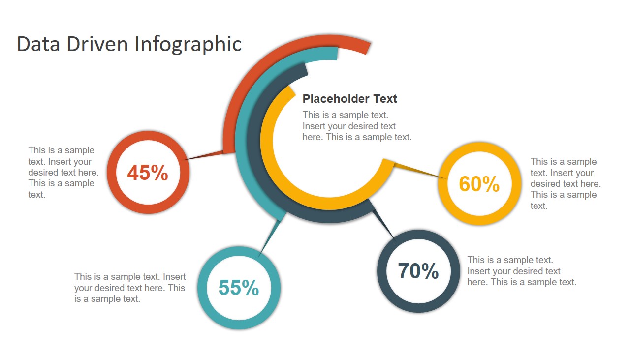
An alternative to the pie chart and donut chart diagrams, this template features a series of curved shapes with bubble callouts as ways of presenting data. Expand the information for each arch in the text placeholder areas.
4. Colorful Metrics Dashboard for Data Presentation

This versatile dashboard template helps us in the presentation of the data by offering several graphs and methods to convert numbers into graphics. Implement it for e-commerce projects, financial projections, project development, and more.
5. Animated Data Presentation Tools for PowerPoint & Google Slides

A slide deck filled with most of the tools mentioned in this article, from bar charts, column charts, treemap graphs, pie charts, histogram, etc. Animated effects make each slide look dynamic when sharing data with stakeholders.
6. Statistics Waffle Charts PPT Template for Data Presentations
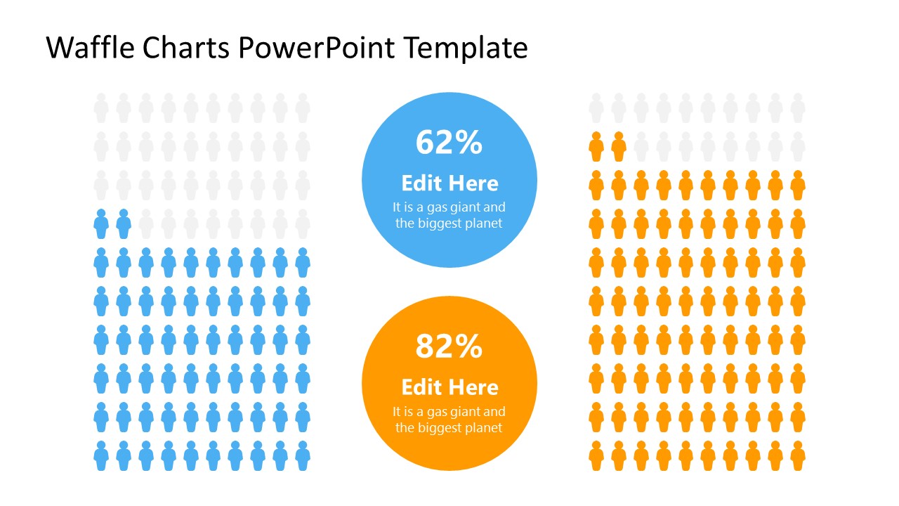
This PPT template helps us how to present data beyond the typical pie chart representation. It is widely used for demographics, so it’s a great fit for marketing teams, data science professionals, HR personnel, and more.
7. Data Presentation Dashboard Template for Google Slides

A compendium of tools in dashboard format featuring line graphs, bar charts, column charts, and neatly arranged placeholder text areas.
8. Weather Dashboard for Data Presentation

Share weather data for agricultural presentation topics, environmental studies, or any kind of presentation that requires a highly visual layout for weather forecasting on a single day. Two color themes are available.
9. Social Media Marketing Dashboard Data Presentation Template

Intended for marketing professionals, this dashboard template for data presentation is a tool for presenting data analytics from social media channels. Two slide layouts featuring line graphs and column charts.
10. Project Management Summary Dashboard Template

A tool crafted for project managers to deliver highly visual reports on a project’s completion, the profits it delivered for the company, and expenses/time required to execute it. 4 different color layouts are available.
11. Profit & Loss Dashboard for PowerPoint and Google Slides
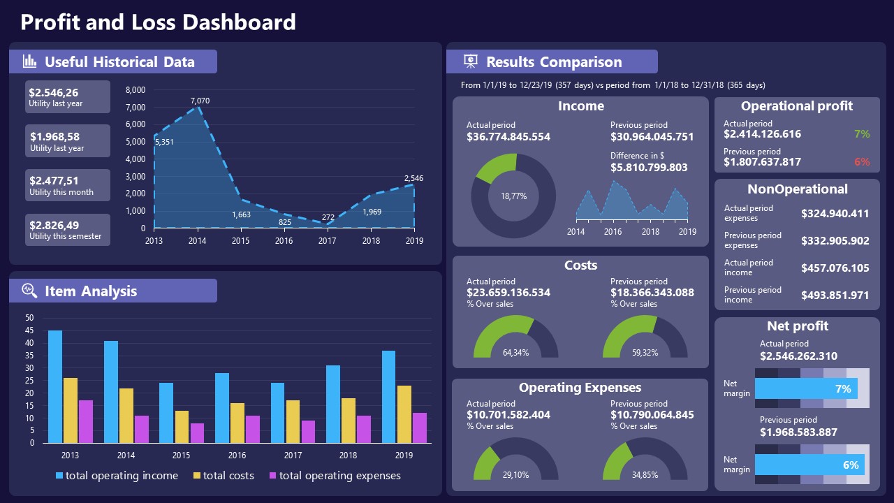
A must-have for finance professionals. This typical profit & loss dashboard includes progress bars, donut charts, column charts, line graphs, and everything that’s required to deliver a comprehensive report about a company’s financial situation.
Overwhelming visuals
One of the mistakes related to using data-presenting methods is including too much data or using overly complex visualizations. They can confuse the audience and dilute the key message.
Inappropriate chart types
Choosing the wrong type of chart for the data at hand can lead to misinterpretation. For example, using a pie chart for data that doesn’t represent parts of a whole is not right.
Lack of context
Failing to provide context or sufficient labeling can make it challenging for the audience to understand the significance of the presented data.
Inconsistency in design
Using inconsistent design elements and color schemes across different visualizations can create confusion and visual disarray.
Failure to provide details
Simply presenting raw data without offering clear insights or takeaways can leave the audience without a meaningful conclusion.
Lack of focus
Not having a clear focus on the key message or main takeaway can result in a presentation that lacks a central theme.
Visual accessibility issues
Overlooking the visual accessibility of charts and graphs can exclude certain audience members who may have difficulty interpreting visual information.
In order to avoid these mistakes in data presentation, presenters can benefit from using presentation templates . These templates provide a structured framework. They ensure consistency, clarity, and an aesthetically pleasing design, enhancing data communication’s overall impact.
Understanding and choosing data presentation types are pivotal in effective communication. Each method serves a unique purpose, so selecting the appropriate one depends on the nature of the data and the message to be conveyed. The diverse array of presentation types offers versatility in visually representing information, from bar charts showing values to pie charts illustrating proportions.
Using the proper method enhances clarity, engages the audience, and ensures that data sets are not just presented but comprehensively understood. By appreciating the strengths and limitations of different presentation types, communicators can tailor their approach to convey information accurately, developing a deeper connection between data and audience understanding.
[1] Government of Canada, S.C. (2021) 5 Data Visualization 5.2 Bar Chart , 5.2 Bar chart . https://www150.statcan.gc.ca/n1/edu/power-pouvoir/ch9/bargraph-diagrammeabarres/5214818-eng.htm
[2] Kosslyn, S.M., 1989. Understanding charts and graphs. Applied cognitive psychology, 3(3), pp.185-225. https://apps.dtic.mil/sti/pdfs/ADA183409.pdf
[3] Creating a Dashboard . https://it.tufts.edu/book/export/html/1870
[4] https://www.goldenwestcollege.edu/research/data-and-more/data-dashboards/index.html
[5] https://www.mit.edu/course/21/21.guide/grf-line.htm
[6] Jadeja, M. and Shah, K., 2015, January. Tree-Map: A Visualization Tool for Large Data. In GSB@ SIGIR (pp. 9-13). https://ceur-ws.org/Vol-1393/gsb15proceedings.pdf#page=15
[7] Heat Maps and Quilt Plots. https://www.publichealth.columbia.edu/research/population-health-methods/heat-maps-and-quilt-plots
[8] EIU QGIS WORKSHOP. https://www.eiu.edu/qgisworkshop/heatmaps.php
[9] About Pie Charts. https://www.mit.edu/~mbarker/formula1/f1help/11-ch-c8.htm
[10] Histograms. https://sites.utexas.edu/sos/guided/descriptive/numericaldd/descriptiven2/histogram/ [11] https://asq.org/quality-resources/scatter-diagram
Like this article? Please share
Data Analysis, Data Science, Data Visualization Filed under Design
Related Articles

Filed under Google Slides Tutorials • June 3rd, 2024
How To Make a Graph on Google Slides
Creating quality graphics is an essential aspect of designing data presentations. Learn how to make a graph in Google Slides with this guide.

Filed under Design • March 27th, 2024
How to Make a Presentation Graph
Detailed step-by-step instructions to master the art of how to make a presentation graph in PowerPoint and Google Slides. Check it out!

Filed under Presentation Ideas • February 12th, 2024
Turning Your Data into Eye-opening Stories
What is Data Storytelling is a question that people are constantly asking now. If you seek to understand how to create a data storytelling ppt that will complete the information for your audience, you should read this blog post.
Leave a Reply
- School Guide
- Mathematics
- Number System and Arithmetic
- Trigonometry
- Probability
- Mensuration
- Maths Formulas
- Class 8 Maths Notes
- Class 9 Maths Notes
- Class 10 Maths Notes
- Class 11 Maths Notes
- Class 12 Maths Notes
Graphical Representation of Data
Graphical Representation of Data: Graphical Representation of Data,” where numbers and facts become lively pictures and colorful diagrams . Instead of staring at boring lists of numbers, we use fun charts, cool graphs, and interesting visuals to understand information better. In this exciting concept of data visualization, we’ll learn about different kinds of graphs, charts, and pictures that help us see patterns and stories hidden in data.
There is an entire branch in mathematics dedicated to dealing with collecting, analyzing, interpreting, and presenting numerical data in visual form in such a way that it becomes easy to understand and the data becomes easy to compare as well, the branch is known as Statistics .
The branch is widely spread and has a plethora of real-life applications such as Business Analytics, demography, Astro statistics, and so on . In this article, we have provided everything about the graphical representation of data, including its types, rules, advantages, etc.

Table of Content
What is Graphical Representation
Types of graphical representations, line graphs, histograms , stem and leaf plot , box and whisker plot .
- Graphical Representations used in Maths
Value-Based or Time Series Graphs
Frequency based, principles of graphical representations, advantages and disadvantages of using graphical system, general rules for graphical representation of data, frequency polygon, solved examples on graphical representation of data.
Graphics Representation is a way of representing any data in picturized form . It helps a reader to understand the large set of data very easily as it gives us various data patterns in visualized form.
There are two ways of representing data,
- Pictorial Representation through graphs.
They say, “A picture is worth a thousand words”. It’s always better to represent data in a graphical format. Even in Practical Evidence and Surveys, scientists have found that the restoration and understanding of any information is better when it is available in the form of visuals as Human beings process data better in visual form than any other form.
Does it increase the ability 2 times or 3 times? The answer is it increases the Power of understanding 60,000 times for a normal Human being, the fact is amusing and true at the same time.
Check: Graph and its representations
Comparison between different items is best shown with graphs, it becomes easier to compare the crux of the data about different items. Let’s look at all the different types of graphical representations briefly:
A line graph is used to show how the value of a particular variable changes with time. We plot this graph by connecting the points at different values of the variable. It can be useful for analyzing the trends in the data and predicting further trends.

A bar graph is a type of graphical representation of the data in which bars of uniform width are drawn with equal spacing between them on one axis (x-axis usually), depicting the variable. The values of the variables are represented by the height of the bars.

This is similar to bar graphs, but it is based frequency of numerical values rather than their actual values. The data is organized into intervals and the bars represent the frequency of the values in that range. That is, it counts how many values of the data lie in a particular range.

It is a plot that displays data as points and checkmarks above a number line, showing the frequency of the point.

This is a type of plot in which each value is split into a “leaf”(in most cases, it is the last digit) and “stem”(the other remaining digits). For example: the number 42 is split into leaf (2) and stem (4).

These plots divide the data into four parts to show their summary. They are more concerned about the spread, average, and median of the data.

It is a type of graph which represents the data in form of a circular graph. The circle is divided such that each portion represents a proportion of the whole.

Graphical Representations used in Math’s
Graphs in Math are used to study the relationships between two or more variables that are changing. Statistical data can be summarized in a better way using graphs. There are basically two lines of thoughts of making graphs in maths:
- Value-Based or Time Series Graphs
These graphs allow us to study the change of a variable with respect to another variable within a given interval of time. The variables can be anything. Time Series graphs study the change of variable with time. They study the trends, periodic behavior, and patterns in the series. We are more concerned with the values of the variables here rather than the frequency of those values.
Example: Line Graph
These kinds of graphs are more concerned with the distribution of data. How many values lie between a particular range of the variables, and which range has the maximum frequency of the values. They are used to judge a spread and average and sometimes median of a variable under study.
Also read: Types of Statistical Data
- All types of graphical representations follow algebraic principles.
- When plotting a graph, there’s an origin and two axes.
- The x-axis is horizontal, and the y-axis is vertical.
- The axes divide the plane into four quadrants.
- The origin is where the axes intersect.
- Positive x-values are to the right of the origin; negative x-values are to the left.
- Positive y-values are above the x-axis; negative y-values are below.

- It gives us a summary of the data which is easier to look at and analyze.
- It saves time.
- We can compare and study more than one variable at a time.
Disadvantages
- It usually takes only one aspect of the data and ignores the other. For example, A bar graph does not represent the mean, median, and other statistics of the data.
- Interpretation of graphs can vary based on individual perspectives, leading to subjective conclusions.
- Poorly constructed or misleading visuals can distort data interpretation and lead to incorrect conclusions.
Check : Diagrammatic and Graphic Presentation of Data
We should keep in mind some things while plotting and designing these graphs. The goal should be a better and clear picture of the data. Following things should be kept in mind while plotting the above graphs:
- Whenever possible, the data source must be mentioned for the viewer.
- Always choose the proper colors and font sizes. They should be chosen to keep in mind that the graphs should look neat.
- The measurement Unit should be mentioned in the top right corner of the graph.
- The proper scale should be chosen while making the graph, it should be chosen such that the graph looks accurate.
- Last but not the least, a suitable title should be chosen.
A frequency polygon is a graph that is constructed by joining the midpoint of the intervals. The height of the interval or the bin represents the frequency of the values that lie in that interval.

Question 1: What are different types of frequency-based plots?
Types of frequency-based plots: Histogram Frequency Polygon Box Plots
Question 2: A company with an advertising budget of Rs 10,00,00,000 has planned the following expenditure in the different advertising channels such as TV Advertisement, Radio, Facebook, Instagram, and Printed media. The table represents the money spent on different channels.
Draw a bar graph for the following data.
- Put each of the channels on the x-axis
- The height of the bars is decided by the value of each channel.

Question 3: Draw a line plot for the following data
- Put each of the x-axis row value on the x-axis
- joint the value corresponding to the each value of the x-axis.

Question 4: Make a frequency plot of the following data:
- Draw the class intervals on the x-axis and frequencies on the y-axis.
- Calculate the midpoint of each class interval.
| Class Interval | Mid Point | Frequency |
| 0-3 | 1.5 | 3 |
| 3-6 | 4.5 | 4 |
| 6-9 | 7.5 | 2 |
| 9-12 | 10.5 | 6 |
Now join the mid points of the intervals and their corresponding frequencies on the graph.

This graph shows both the histogram and frequency polygon for the given distribution.
Related Article:
Graphical Representation of Data| Practical Work in Geography Class 12 What are the different ways of Data Representation What are the different ways of Data Representation? Charts and Graphs for Data Visualization
Conclusion of Graphical Representation
Graphical representation is a powerful tool for understanding data, but it’s essential to be aware of its limitations. While graphs and charts can make information easier to grasp, they can also be subjective, complex, and potentially misleading . By using graphical representations wisely and critically, we can extract valuable insights from data, empowering us to make informed decisions with confidence.
Graphical Representation of Data – FAQs
What are the advantages of using graphs to represent data.
Graphs offer visualization, clarity, and easy comparison of data, aiding in outlier identification and predictive analysis.
What are the common types of graphs used for data representation?
Common graph types include bar, line, pie, histogram, and scatter plots , each suited for different data representations and analysis purposes.
How do you choose the most appropriate type of graph for your data?
Select a graph type based on data type, analysis objective, and audience familiarity to effectively convey information and insights.
How do you create effective labels and titles for graphs?
Use descriptive titles, clear axis labels with units, and legends to ensure the graph communicates information clearly and concisely.
How do you interpret graphs to extract meaningful insights from data?
Interpret graphs by examining trends, identifying outliers, comparing data across categories, and considering the broader context to draw meaningful insights and conclusions.
Please Login to comment...
Similar reads.
- School Learning
- Maths-Class-9
Improve your Coding Skills with Practice
What kind of Experience do you want to share?
Call Us Today! +91 99907 48956 | [email protected]
It is the simplest form of data Presentation often used in schools or universities to provide a clearer picture to students, who are better able to capture the concepts effectively through a pictorial Presentation of simple data.
2. Column chart

It is a simplified version of the pictorial Presentation which involves the management of a larger amount of data being shared during the presentations and providing suitable clarity to the insights of the data.
3. Pie Charts

Pie charts provide a very descriptive & a 2D depiction of the data pertaining to comparisons or resemblance of data in two separate fields.
4. Bar charts

A bar chart that shows the accumulation of data with cuboid bars with different dimensions & lengths which are directly proportionate to the values they represent. The bars can be placed either vertically or horizontally depending on the data being represented.
5. Histograms
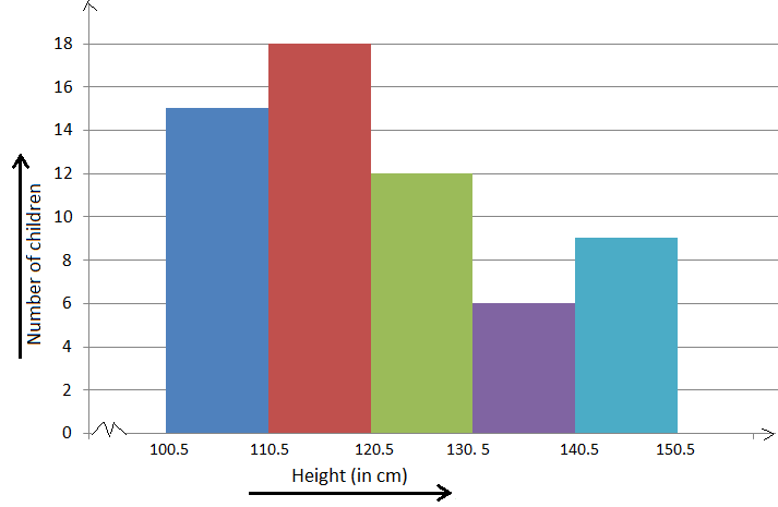
It is a perfect Presentation of the spread of numerical data. The main differentiation that separates data graphs and histograms are the gaps in the data graphs.
6. Box plots

Box plot or Box-plot is a way of representing groups of numerical data through quartiles. Data Presentation is easier with this style of graph dealing with the extraction of data to the minutes of difference.

Map Data graphs help you with data Presentation over an area to display the areas of concern. Map graphs are useful to make an exact depiction of data over a vast case scenario.
All these visual presentations share a common goal of creating meaningful insights and a platform to understand and manage the data in relation to the growth and expansion of one’s in-depth understanding of data & details to plan or execute future decisions or actions.
Importance of Data Presentation
Data Presentation could be both can be a deal maker or deal breaker based on the delivery of the content in the context of visual depiction.
Data Presentation tools are powerful communication tools that can simplify the data by making it easily understandable & readable at the same time while attracting & keeping the interest of its readers and effectively showcase large amounts of complex data in a simplified manner.
If the user can create an insightful presentation of the data in hand with the same sets of facts and figures, then the results promise to be impressive.
There have been situations where the user has had a great amount of data and vision for expansion but the presentation drowned his/her vision.
To impress the higher management and top brass of a firm, effective presentation of data is needed.
Data Presentation helps the clients or the audience to not spend time grasping the concept and the future alternatives of the business and to convince them to invest in the company & turn it profitable both for the investors & the company.
Although data presentation has a lot to offer, the following are some of the major reason behind the essence of an effective presentation:-
- Many consumers or higher authorities are interested in the interpretation of data, not the raw data itself. Therefore, after the analysis of the data, users should represent the data with a visual aspect for better understanding and knowledge.
- The user should not overwhelm the audience with a number of slides of the presentation and inject an ample amount of texts as pictures that will speak for themselves.
- Data presentation often happens in a nutshell with each department showcasing their achievements towards company growth through a graph or a histogram.
- Providing a brief description would help the user to attain attention in a small amount of time while informing the audience about the context of the presentation
- The inclusion of pictures, charts, graphs and tables in the presentation help for better understanding the potential outcomes.
- An effective presentation would allow the organization to determine the difference with the fellow organization and acknowledge its flaws. Comparison of data would assist them in decision making.
Recommended Courses

Data Visualization
Using powerbi &tableau.

Tableau for Data Analysis

MySQL Certification Program
The PowerBI Masterclass
Need help call our support team 7:00 am to 10:00 pm (ist) at (+91 999-074-8956 | 9650-308-956), keep in touch, email: [email protected].
WhatsApp us
Computer Network
- Operating Systems
- Computer Fundamentals
- Interview Q
Physical Layer
Data link layer, network layer, routing algorithm, transport layer, application layer, application protocols, network security.
Interview Questions

| A network is a collection of different devices connected and capable of communicating. For example, a company's local network connects employees' computers and devices like printers and scanners. Employees will be able to share information using the network and also use the common printer/ scanner via the network. Data to be transferred or communicated from one device to another comes in various formats like audio, video, etc. This tutorial explains how different data types are represented in a computer and transferred in a network.
Data in text format is represented using bit patterns (combinations of two binary bits - 0 and 1). Textual data is nothing but a string, and a string is a collection of characters. Each character is given a specific number according to an international standard called Unicode. The process of allocating numbers to characters is called "Coding," and these numbers are called "codes". Now, these codes are converted into binary bits to represent the textual data in a pattern of bits, and these bits are transferred as a stream via the network to other devices.
It is the universal standard of character encoding. It gives a unique code to almost all the characters in every language spoken in the world. It defines more than 1 40 000 characters. It even defined codes for emojis. The first 128 characters of Unicode point to ASCII characters. ASCII is yet another character encoding format, but it has only 128 codes to 128 characters. Hence, ASCII is a subset of Unicode.
.doc, .docx, .pdf, .txt, etc.
Word: H Unicode representation: U+0048 Numbers are directly converted into binary patterns by dividing by 2 without any encoding. The numbers we want to transfer generally will be of the decimal number system- ( ) . We need to convert the numbers from ( ) to a binary number system - ( )
Integers Date Boolean Decimal Fixed point Floating point
Number: 780 Binary representation: 1100001100 Image data is also transferred as a stream of bits like textual data. An image, also called a picture, is a collection of little elements called " ". A single pixel is the smallest addressable element of a picture, and it is like a dot with a size of 1/96 inch/ 0.26 mm. The dimensions of an image are given by the
A black-and-white/ Grayscale image consists of white, black, and all the shades in between. It can be considered as just . The intensity of the white color in a pixel is given by numbers called " ". The pixel value in a Grayscale image can be in the range , where 0 represents Black and 255 represents White, and all the numbers in the interval represent different shades. A matrix is created for the image with pixel values of all the pixels in the image. This matrix is called a " ".
representing three standard colors: . Any color known can be generated by using these three colors. Based on the intensity of a color in the pixel, three matrices/ channels for each color are generated. Suppose there is a colored image, and three matrices are created for Red, Green, and Blue colors in each pixel in the image: , and this bit stream is transferred to any other device in the network to communicate the image. N-bit streams are used to represent 2N possible colors. From 0 to 255, we can represent 256 shades of color with different 8-bit patterns. , an image consists of only either black or white colors, only one bit will be enough to represent the pixels: White - 1 Black - 0
.jpg, jpeg, .png, etc. Transferring an audio signal is different from other formats. Audio is broadcasting recorded sound or music. An audio signal is to be stored in a computer by representing the wave amplitude at moments in bits. Another parameter is the sample rate. It represents the number of samples or, in other words, samples saved. The audio quality depends and the . If more bits are used to represent the amplitudes in moments and more moments are captured accurately, we can save the audio with every detail accurately.
.mp3, .m4a, .WAV, .AAC, etc. A video is a with the same or different dimensions. These frames/ images are represented as matrices, as we discussed above. All the frames/ images are displayed continuously, one after the other, to show a video in movement. To represent a video, The computer will analyze data about the video like: (Frames per second)A video is mostly combined with an audio component, like a film or a video game.
.mp4, .MOV, .AVI, etc. |

- Send your Feedback to [email protected]
Help Others, Please Share

Learn Latest Tutorials

Transact-SQL

Reinforcement Learning

R Programming

React Native

Python Design Patterns

Python Pillow

Python Turtle

Preparation

Verbal Ability
Company Questions
Trending Technologies

Artificial Intelligence

Cloud Computing

Data Science

Machine Learning

B.Tech / MCA

Data Structures

Operating System

Compiler Design

Computer Organization

Discrete Mathematics

Ethical Hacking

Computer Graphics

Software Engineering

Web Technology

Cyber Security

C Programming

Control System

Data Mining

Data Warehouse

CHEPLASKEI BOYS HIGH SCHOOL
Types of data representation.
- Computers not only process numbers, letters and special symbols but also complex types of data such as sound and pictures. However, these complex types of data take a lot of memory and processor time when coded in binary form.
- This limitation necessitates the need to develop better ways of handling long streams of binary digits.
Number systems and their representation
- A number system is a set of symbols used to represent values derived from a common base or radix.
- As far as computers are concerned, number systems can be classified into two major categories:
- decimal number system
- binary number system
- octal number system
- hexadecimal number system
Decimal number system
- The term decimal is derived from a Latin prefix deci, which means ten. Decimal number system has ten digits ranging from 0-9. Because this system has ten digits; it is also called a base ten number system or denary number system.
- A decimal number should always be written with a subscript 10 e.g. X 10
- But since this is the most widely used number system in the world, the subscript is usually understood and ignored in written work. However ,when many number systems are considered together, the subscript must always be put so as to differentiate the number systems.
- The magnitude of a number can be considered using these parameters.
- Absolute value
- Place value or positional value
- The absolute value is the magnitude of a digit in a number. for example the digit 5 in 7458 has an absolute value of 5 according to its value in the number line.
- The place value of a digit in a number refers to the position of the digit in that number i.e. whether; tens, hundreds, thousands etc.
- The total value of a number is the sum of the place value of each digit making the number.
- The base value of a number also k known as the radix , depends on the type of the number systems that is being used .The value of any number depends on the radix. for example the number 100 10 is not equivalent to 100 2 .
Thank you for visiting nature.com. You are using a browser version with limited support for CSS. To obtain the best experience, we recommend you use a more up to date browser (or turn off compatibility mode in Internet Explorer). In the meantime, to ensure continued support, we are displaying the site without styles and JavaScript.
- View all journals
- Explore content
- About the journal
- Publish with us
- Sign up for alerts
- Open access
- Published: 21 August 2024
Loss of plasticity in deep continual learning
- Shibhansh Dohare ORCID: orcid.org/0000-0002-3796-9347 1 ,
- J. Fernando Hernandez-Garcia 1 ,
- Qingfeng Lan ORCID: orcid.org/0000-0001-8568-7603 1 ,
- Parash Rahman ORCID: orcid.org/0000-0001-8430-2679 1 ,
- A. Rupam Mahmood ORCID: orcid.org/0000-0001-6266-162X 1 , 2 &
- Richard S. Sutton 1 , 2
Nature volume 632 , pages 768–774 ( 2024 ) Cite this article
3074 Accesses
91 Altmetric
Metrics details
- Computer science
- Human behaviour
Artificial neural networks, deep-learning methods and the backpropagation algorithm 1 form the foundation of modern machine learning and artificial intelligence. These methods are almost always used in two phases, one in which the weights of the network are updated and one in which the weights are held constant while the network is used or evaluated. This contrasts with natural learning and many applications, which require continual learning. It has been unclear whether or not deep learning methods work in continual learning settings. Here we show that they do not—that standard deep-learning methods gradually lose plasticity in continual-learning settings until they learn no better than a shallow network. We show such loss of plasticity using the classic ImageNet dataset and reinforcement-learning problems across a wide range of variations in the network and the learning algorithm. Plasticity is maintained indefinitely only by algorithms that continually inject diversity into the network, such as our continual backpropagation algorithm, a variation of backpropagation in which a small fraction of less-used units are continually and randomly reinitialized. Our results indicate that methods based on gradient descent are not enough—that sustained deep learning requires a random, non-gradient component to maintain variability and plasticity.
Inferring neural activity before plasticity as a foundation for learning beyond backpropagation

Three types of incremental learning

Meta-learning biologically plausible plasticity rules with random feedback pathways
Machine learning and artificial intelligence have made remarkable progress in the past decade, with landmark successes in natural-language processing 2 , 3 , biology 4 , game playing 5 , 6 , 7 , 8 and robotics 9 , 10 . All these systems use artificial neural networks, whose computations are inspired by the operation of human and animal brains. Learning in these networks refers to computational algorithms for changing the strengths of their connection weights (computational synapses). The most important modern learning methods are based on stochastic gradient descent (SGD) and the backpropagation algorithm, ideas that originated at least four decades ago but are much more powerful today because of the availability of vastly greater computer power. The successes are also because of refinements of the learning and training techniques that together make the early ideas effective in much larger and more deeply layered networks. These methodologies are collectively referred to as deep learning.
Despite its successes, deep learning has difficulty adapting to changing data. Because of this, in almost all applications, deep learning is restricted to a special training phase and then turned off when the network is actually used. For example, large language models such as ChatGPT are trained on a large generic training set and then fine-tuned on smaller datasets specific to an application or to meet policy and safety goals, but finally their weights are frozen before the network is released for use. With current methods, it is usually not effective to simply continue training on new data when they become available. The effect of the new data is either too large or too small and not properly balanced with the old data. The reasons for this are not well understood and there is not yet a clear solution. In practice, the most common strategy for incorporating substantial new data has been simply to discard the old network and train a new one from scratch on the old and new data together 11 , 12 . When the network is a large language model and the data are a substantial portion of the internet, then each retraining may cost millions of dollars in computation. Moreover, a wide range of real-world applications require adapting to change. Change is ubiquitous in learning to anticipate markets and human preferences and in gaming, logistics and control systems. Deep-learning systems would be much more powerful if they, like natural-learning systems, were capable of continual learning.
Here we show systematically that standard deep-learning methods lose their ability to learn with extended training on new data, a phenomenon that we call loss of plasticity. We use classic datasets, such as ImageNet and CIFAR-100, modified for continual learning, and standard feed-forward and residual networks with a wide variety of standard learning algorithms. Loss of plasticity in artificial neural networks was first shown at the turn of the century in the psychology literature 13 , 14 , 15 , before the development of deep-learning methods. Plasticity loss with modern methods was visible in some recent works 11 , 16 , 17 , 18 and most recently has begun to be explored explicitly 12 , 19 , 20 , 21 , 22 , 23 , 24 , 25 , 26 , 27 . Loss of plasticity is different from catastrophic forgetting, which concerns poor performance on old examples even if they are not presented again 28 , 29 , 30 .
Although standard deep-learning methods lose plasticity with extended learning, we show that a simple change enables them to maintain plasticity indefinitely in both supervised and reinforcement learning. Our new algorithm, continual backpropagation, is exactly like classical backpropagation except that a tiny proportion of less-used units are reinitialized on each step much as they were all initialized at the start of training. Continual backpropagation is inspired by a long history of methods for automatically generating and testing features, starting with Selfridge’s Pandemonium in 1959 (refs. 19 , 20 , 31 , 32 , 33 , 34 , 35 ). The effectiveness of continual backpropagation shows that the problem of plasticity loss is not inherent in artificial neural networks.
Plasticity loss in supervised learning
The primary purpose of this article is to demonstrate loss of plasticity in standard deep-learning systems. For the demonstration to be convincing, it must be systematic and extensive. It must consider a wide range of standard deep-learning networks, learning algorithms and parameter settings. For each of these, the experiments must be run long enough to expose long-term plasticity loss and be repeated enough times to obtain statistically significant results. Altogether, more computation is needed by three or four orders of magnitude compared with what would be needed to train a single network. For example, a systematic study with large language models would not be possible today because just a single training run with one of these networks would require computation costing millions of dollars. Fortunately, advances in computer hardware have continued apace since the development of deep learning and systematic studies have become possible with the deep-learning networks used earlier and with some of the longer-lived test problems. Here we use ImageNet, a classic object-recognition test bed 36 , which played a pivotal role in the rise of deep learning 37 and is still influential today.
The ImageNet database comprises millions of images labelled by nouns (classes) such as types of animal and everyday object. The typical ImageNet task is to guess the label given an image. The standard way to use this dataset is to partition it into training and test sets. A learning system is first trained on a set of images and their labels, then training is stopped and performance is measured on a separate set of test images from the same classes. To adapt ImageNet to continual learning while minimizing all other changes, we constructed a sequence of binary classification tasks by taking the classes in pairs. For example, the first task might be to distinguish cats from houses and the second might be to distinguish stop signs from school buses. With the 1,000 classes in our dataset, we were able to form half a million binary classification tasks in this way. For each task, a deep-learning network was first trained on a subset of the images for the two classes and then its performance was measured on a separate test set for the classes. After training and testing on one task, the next task began with a different pair of classes. We call this problem ‘Continual ImageNet’. In Continual ImageNet, the difficulty of tasks remains the same over time. A drop in performance would mean the network is losing its learning ability, a direct demonstration of loss of plasticity.
We applied a wide variety of standard deep-learning networks to Continual ImageNet and tested many learning algorithms and parameter settings. To assess the performance of the network on a task, we measured the percentage of test images that were correctly classified. The results shown in Fig. 1b are representative; they are for a feed-forward convolutional network and for a training procedure, using unmodified backpropagation, that performed well on this problem in the first few tasks.

a – c , In a sequence of binary classification tasks using ImageNet pictures ( a ), the conventional backpropagation algorithm loses plasticity at all step sizes ( b ), whereas the continual backpropagation, L2 regularization and Shrink and Perturb algorithms maintain plasticity, apparently indefinitely ( c ). All results are averaged over 30 runs; the solid lines represent the mean and the shaded regions correspond to ±1 standard error.
Although these networks learned up to 88% correct on the test set of the early tasks (Fig. 1b , left panel), by the 2,000th task, they had lost substantial plasticity for all values of the step-size parameter (right panel). Some step sizes performed well on the first two tasks but then much worse on subsequent tasks, eventually reaching a performance level below that of a linear network. For other step sizes, performance rose initially and then fell and was only slightly better than the linear network after 2,000 tasks. We found this to be a common pattern in our experiments: for a well-tuned network, performance first improves and then falls substantially, ending near or below the linear baseline. We have observed this pattern for many network architectures, parameter choices and optimizers. The specific choice of network architecture, algorithm parameters and optimizers affected when the performance started to drop, but a severe performance drop occurred for a wide range of choices. The failure of standard deep-learning methods to learn better than a linear network in later tasks is direct evidence that these methods do not work well in continual-learning problems.
Algorithms that explicitly keep the weights of the network small were an exception to the pattern of failure and were often able to maintain plasticity and even improve their performance over many tasks, as shown in Fig. 1c . L2 regularization adds a penalty for large weights; augmenting backpropagation with this enabled the network to continue improving its learning performance over at least 5,000 tasks. The Shrink and Perturb algorithm 11 , which includes L2 regularization, also performed well. Best of all was our continual backpropagation algorithm, which we discuss later. For all algorithms, we tested a wide range of parameter settings and performed many independent runs for statistical significance. The presented curves are the best representative of each algorithm.
For a second demonstration, we chose to use residual networks, class-incremental continual learning and the CIFAR-100 dataset. Residual networks include layer-skipping connections as well as the usual layer-to-layer connections of conventional convolutional networks. The residual networks of today are more widely used and produce better results than strictly layered networks 38 . Class-incremental continual learning 39 involves sequentially adding new classes while testing on all classes seen so far. In our demonstration, we started with training on five classes and then successively added more, five at a time, until all 100 were available. After each addition, the networks were trained and performance was measured on all available classes. We continued training on the old classes (unlike in most work in class-incremental learning) to focus on plasticity rather than on forgetting.
In this demonstration, we used an 18-layer residual network with a variable number of heads, adding heads as new classes were added. We also used further deep-learning techniques, including batch normalization, data augmentation, L2 regularization and learning-rate scheduling. These techniques are standardly used with residual networks and are necessary for good performance. We call this our base deep-learning system.
As more classes are added, correctly classifying images becomes more difficult and classification accuracy would decrease even if the network maintained its ability to learn. To factor out this effect, we compare the accuracy of our incrementally trained networks with networks that were retrained from scratch on the same subset of classes. For example, the network that was trained first on five classes, and then on all ten classes, is compared with a network retrained from scratch on all ten classes. If the incrementally trained network performs better than a network retrained from scratch, then there is a benefit owing to training on previous classes, and if it performs worse, then there is genuine loss of plasticity.
The red line in Fig. 2b shows that incremental training was initially better than retraining, but after 40 classes, the incrementally trained network showed loss of plasticity that became increasingly severe. By the end, when all 100 classes were available, the accuracy of the incrementally trained base system was 5% lower than the retrained network (a performance drop equivalent to that of removing a notable algorithmic advance, such as batch normalization). Loss of plasticity was less severe when Shrink and Perturb was added to the learning algorithm (in the incrementally trained network) and was eliminated altogether when continual backpropagation (see the ‘Maintaining plasticity through variability and selective preservation’ section) was added. These additions also prevented units of the network from becoming inactive or redundant, as shown in Fig. 2c,d .

a , An incrementally growing image-classification problem. b , Initially, accuracy is improved by incremental training compared with a network trained from scratch, but after 40 classes, accuracy degrades substantially in a base deep-learning system, less so for a Shrink and Perturb learning system and not at all for a learning system based on continual backpropagation. c , The number of network units that are active less than 1% of the time increases rapidly for the base deep-learning system, but less so for Shrink and Perturb and continual backpropagation systems. d , A low stable rank means that the units of a network do not provide much diversity; the base deep-learning system loses much more diversity than the Shrink and Perturb and continual backpropagation systems. All results are averaged over 30 runs; the solid lines represent the mean and the shaded regions correspond to ±1 standard error.
This demonstration involved larger networks and required more computation, but still we were able to perform extensive systematic tests. We found a robust pattern in the results that was similar to what we found in ImageNet. In both cases, deep-learning networks exhibited substantial loss of plasticity. Altogether, these results, along with other extensive results in Methods , constitute substantial evidence of plasticity loss.
Plasticity loss in reinforcement learning
Continual learning is essential to reinforcement learning in ways that go beyond its importance in supervised learning. Not only can the environment change but the behaviour of the learning agent can also change, thereby influencing the data it receives even if the environment is stationary. For this reason, the need for continual learning is often more apparent in reinforcement learning, and reinforcement learning is an important setting in which to demonstrate the tendency of deep learning towards loss of plasticity.
Nevertheless, it is challenging to demonstrate plasticity loss in reinforcement learning in a systematic and rigorous way. In part, this is because of the great variety of algorithms and experimental settings that are commonly used in reinforcement-learning research. Algorithms may learn value functions, behaviours or both simultaneously and may involve replay buffers, world models and learned latent states. Experiments may be episodic, continuing or offline. All of these choices involve several embedded choices of parameters. More fundamentally, reinforcement-learning algorithms affect the data seen by the agent. The learning ability of an algorithm is thus confounded with its ability to generate informative data. Finally, and in part because of the preceding, reinforcement-learning results tend to be more stochastic and more widely varying than in supervised learning. Altogether, demonstration of reinforcement-learning abilities, particularly negative results, tends to require more runs and generally much more experimental work and thus inevitably cannot be as definitive as in supervised learning.
Our first demonstration involves a reinforcement-learning algorithm applied to a simulated ant-like robot tasked with moving forwards as rapidly and efficiently as possible. The agent–environment interaction comprises a series of episodes, each beginning in a standard state and lasting up to 1,000 time steps. On each time step, the agent receives a reward depending on the forward distance travelled and the magnitude of its action (see Methods for details). An episode terminates in fewer than 1,000 steps if the ant jumps too high instead of moving forwards, as often happens early in learning. In the results to follow, we use the cumulative reward during an episode as our primary performance measure. To make the task non-stationary (and thereby emphasize plasticity), the coefficient of friction between the feet of the ant and the floor is changed after every 2 million time steps (but only at an episode boundary; details in Methods ). For fastest walking, the agent must adapt (relearn) its way of walking each time the friction changes. For this experiment, we used the proximal policy optimization (PPO) algorithm 40 . PPO is a standard deep reinforcement-learning algorithm based on backpropagation. It is widely used, for example, in robotics 9 , in playing real-time strategy games 41 and in aligning large language models from human feedback 42 .
PPO performed well (see the red line in Fig. 3c ) for the first 2 million steps, up until the first change in friction, but then performed worse and worse. Note how the performance of the other algorithms in Fig. 3c decreased each time the friction changed and then recovered as the agent adapted to the new friction, giving the plot a sawtooth appearance. PPO augmented with a specially tuned Adam optimizer 24 , 43 performed much better (orange line in Fig. 3c ) but still performed much worse over successive changes after the first two, indicating substantial loss of plasticity. On the other hand, PPO augmented with L2 regularization and continual backpropagation largely maintained their plasticity as the problem changed.

a , The reinforcement-learning agent controls torques at the eight joints of the simulated ant (red circles) to maximize forward motion and minimize penalties. b , Here we use a version of the ant problem in which the friction on contact with the ground is abruptly changed every 2 million time steps. c , The standard PPO learning algorithm fails catastrophically on the non-stationary ant problem. If the optimizer of PPO (Adam) is tuned in a custom way, then the failure is less severe, but adding continual backpropagation or L2 regularization is necessary to perform well indefinitely. These results are averaged over 100 runs; the solid lines represent the mean and the shaded regions represent the 95% bootstrapped confidence interval.
Now consider the same ant-locomotion task except with the coefficient of friction held constant at an intermediate value over 50 million time steps. The red line in Fig. 4a shows that the average performance of PPO increased for about 3 million steps but then collapsed. After 20 million steps, the ant is failing every episode and is unable to learn to move forwards efficiently. The red lines in the other panels of Fig. 4 provide further insight into the loss of plasticity of PPO. They suggest that the network may be losing plasticity in the same way as in our supervised learning results (see Fig. 2 and Extended Data Fig. 3c ). In both cases, most of the network’s units became dormant during the experiment, and the network markedly lost stable rank. The addition of L2 regularization mitigated the performance degradation by preventing continual growth of weights but also resulted in very small weights (Fig. 4d ), which prevented the agent from committing to good behaviour. The addition of continual backpropagation performed better overall. We present results for continual backpropagation only with (slight) L2 regularization, because without it, performance was highly sensitive to parameter settings. These results show that plasticity loss can be catastrophic in both deep reinforcement learning as well as deep supervised learning.

a , The four reinforcement-learning algorithms performed similarly on this and the non-stationary problem (compare with Fig. 3c ). b , c , A closer look inside the networks reveals a similar pattern as in supervised learning (compare with Fig. 2c,d ). d , The absolute values of the weights of the networks increased steadily under standard and tuned PPO, whereas they decreased and stayed small under L2 regularization with or without continual backpropagation. These results are averaged over 30 runs; the solid lines represent the mean and the shaded regions represent the 95% bootstrapped confidence interval.
Maintaining plasticity
Surprisingly, popular methods such as Adam, Dropout and normalization actually increased loss of plasticity (see Extended Data Fig. 4a ). L2 regularization, on the other hand, reduced loss of plasticity in many cases (purple line in Figs. 1 , 3 and 4 ). L2 regularization stops the weights from becoming too large by moving them towards zero at each step. The small weights allow the network to remain plastic. Another existing method that reduced loss of plasticity is Shrink and Perturb 11 (orange line in Figs. 1 and 2 ). Shrink and Perturb is L2 regularization plus small random changes in weights at each step. The injection of variability into the network can reduce dormancy and increase the diversity of the representation (Figs. 2 and 4 ). Our results indicate that non-growing weights and sustained variability in the network may be important for maintaining plasticity.
We now describe a variation of the backpropagation algorithm that is explicitly designed to inject variability into the network and keep some of its weights small. Conventional backpropagation has two main parts: initialization with small random weights before training and then gradient descent at each training step. The initialization provides variability initially, but, as we have seen, with continued training, variability tends to be lost, as well as plasticity along with it. To maintain the variability, our new algorithm, continual backpropagation, reinitializes a small number of units during training, typically fewer than one per step. To prevent disruption of what the network has already learned, only the least-used units are considered for reinitialization. See Methods for details.
The blue line in Fig. 1c shows the performance of continual backpropagation on Continual ImageNet. It mitigated loss of plasticity in Continual ImageNet while outperforming existing methods. Similarly, the blue lines in Fig. 2 show the performance of continual backpropagation on class-incremental CIFAR-100 and its effect on the evolution of dormant units and stable rank. Continual backpropagation fully overcame loss of plasticity, with a high stable rank and almost no dead units throughout learning.
In reinforcement learning, continual backpropagation was applied together with L2 regularization (a small amount of regularization was added to prevent excessive sensitivity to parameters in reinforcement-learning experiments). The blue line in Fig. 3 shows the performance of PPO with continual backpropagation on the ant-locomotion problem with changing friction. PPO with continual backpropagation performed much better than standard PPO, with little or no loss of plasticity. On the ant-locomotion problem with constant friction (Fig. 4 ), PPO with continual backpropagation continued improving throughout the experiment. The blue lines in Fig. 4b–d show the evolution of the correlates of loss of plasticity when we used continual backpropagation. PPO with continual backpropagation had few dormant units, a high stable rank and an almost constant average weight magnitude.
Our results are consistent with the idea that small weights reduce loss of plasticity and that a continual injection of variability further mitigates loss of plasticity. Although Shrink and Perturb adds variability to all weights, continual backpropagation does so selectively, and this seems to enable it to better maintain plasticity. Continual backpropagation involves a form of variation and selection in the space of neuron-like units, combined with continuing gradient descent. The variation and selection is reminiscent of trial-and-error processes in evolution and behaviour 44 , 45 , 46 , 47 and has precursors in many earlier ideas, including Keifer–Wolfowitz methods 48 and restart methods 49 in engineering and feature-search methods in machine learning 31 , 32 , 33 , 34 , 35 , 50 . Continual backpropagation brings a form of this old idea to modern deep learning. However, it is just one variation of this idea; other variations are possible and some of these have been explored in recent work 25 , 27 . We look forward to future work that explicitly compares and further refines these variations.
Deep learning is an effective and valuable technology in settings in which learning occurs in a special training phase and not thereafter. In settings in which learning must continue, however, we have shown that deep learning does not work. By deep learning, we mean the existing standard algorithms for learning in multilayer artificial neural networks and by not work, we mean that, over time, they fail to learn appreciably better than shallow networks. We have shown such loss of plasticity using supervised-learning datasets and reinforcement-learning tasks on which deep learning has previously excelled and for a wide range of networks and standard learning algorithms. Taking a closer look, we found that, during training, many of the networks’ neuron-like units become dormant, overcommitted and similar to each other, hampering the ability of the networks to learn new things. As they learn, standard deep-learning networks gradually and irreversibly lose their diversity and thus their ability to continue learning. Plasticity loss is often severe when learning continues for many tasks, but may not occur at all for small numbers of tasks.
The problem of plasticity loss is not intrinsic to deep learning. Deep artificial neural networks trained by gradient descent are perfectly capable of maintaining their plasticity, apparently indefinitely, as we have shown with the Shrink and Perturb algorithm and particularly with the new continual backpropagation algorithm. Both of these algorithms extend standard deep learning by adding a source of continuing variability to the weights of the network, and continual backpropagation restricts this variability to the units of the network that are at present least used, minimizing damage to the operation of the network. That is, continual backpropagation involves a form of variation and selection in the space of neuron-like units, combined with continuing gradient descent. This idea has many historical antecedents and will probably require further development to reach its most effective form.
Specifics of continual backpropagation
Continual backpropagation selectively reinitializes low-utility units in the network. Our utility measure, called the contribution utility, is defined for each connection or weight and each unit. The basic intuition behind the contribution utility is that the magnitude of the product of units’ activation and outgoing weight gives information about how valuable this connection is to its consumers. If the contribution of a hidden unit to its consumer is small, its contribution can be overwhelmed by contributions from other hidden units. In such a case, the hidden unit is not useful to its consumer. We define the contribution utility of a hidden unit as the sum of the utilities of all its outgoing connections. The contribution utility is measured as a running average of instantaneous contributions with a decay rate, η , which is set to 0.99 in all experiments. In a feed-forward neural network, the contribution utility, u l [ i ], of the i th hidden unit in layer l at time t is updated as
in which h l , i , t is the output of the i th hidden unit in layer l at time t , w l , i , k , t is the weight connecting the i th unit in layer l to the k th unit in layer l + 1 at time t and n l +1 is the number of units in layer l + 1.
When a hidden unit is reinitialized, its outgoing weights are initialized to zero. Initializing the outgoing weights as zero ensures that the newly added hidden units do not affect the already learned function. However, initializing the outgoing weight to zero makes the new unit vulnerable to immediate reinitialization, as it has zero utility. To protect new units from immediate reinitialization, they are protected from a reinitialization for maturity threshold m number of updates. We call a unit mature if its age is more than m . Every step, a fraction of mature units ρ , called the replacement rate, is reinitialized in every layer.
The replacement rate ρ is typically set to a very small value, meaning that only one unit is replaced after hundreds of updates. For example, in class-incremental CIFAR-100 (Fig. 2 ) we used continual backpropagation with a replacement rate of 10 −5 . The last layer of the network in that problem had 512 units. At each step, roughly 512 × 10 −5 = 0.00512 units are replaced. This corresponds to roughly one replacement after every 1/0.00512 ≈ 200 updates or one replacement after every eight epochs on the first five classes.
The final algorithm combines conventional backpropagation with selective reinitialization to continually inject random units from the initial distribution. Continual backpropagation performs a gradient descent and selective reinitialization step at each update. Algorithm 1 specifies continual backpropagation for a feed-forward neural network. In cases in which the learning system uses mini-batches, the instantaneous contribution utility can be used by averaging the utility over the mini-batch instead of keeping a running average to save computation (see Extended Data Fig. 5d for an example). Continual backpropagation overcomes the limitation of previous work 34 , 35 on selective reinitialization and makes it compatible with modern deep learning.
Algorithm 1
Continual backpropagation for a feed-forward network with L layers
Set replacement rate ρ , decay rate η and maturity threshold m
Initialize the weights w 0 ,…, w L −1 , in which w l is sampled from distribution d l
Initialize utilities u 1 ,…, u L −1 , number of units to replace c 1 ,…, c L −1 , and ages a 1 ,…, a L −1 to 0
For each input x t do
Forward pass: pass x t through the network to get the prediction \(\widehat{{{\bf{y}}}_{t}}\)
Evaluate: receive loss \(l({{\bf{x}}}_{t},\widehat{{{\bf{y}}}_{t}})\)
Backward pass: update the weights using SGD or one of its variants
For layer l in 1: L − 1 do
Update age: a l = a l + 1
Update unit utility: see equation ( 1 )
Find eligible units: n eligible = number of units with age greater than m
Update number of units to replace: c l = c l + n eligible × ρ
If c l > 1
Find the unit with smallest utility and record its index as r
Reinitialize input weights: resample w l −1 [:, r ] from distribution d l
Reinitialize output weights: set w l [ r ,:] to 0
Reinitialize utility and age: set u l [ r ] = 0 and a l [ r ] = 0
Update number of units to replace: c l = c l − 1
Details of Continual ImageNet
The ImageNet database we used consists of 1,000 classes, each of 700 images. The 700 images for each class were divided into 600 images for a training set and 100 images for a test set. On each binary classification task, the deep-learning network was first trained on the training set of 1,200 images and then its classification accuracy was measured on the test set of 200 images. The training consisted of several passes through the training set, called epochs. For each task, all learning algorithms performed 250 passes through the training set using mini-batches of size 100. All tasks used the downsampled 32 × 32 version of the ImageNet dataset, as is often done to save computation 51 .
All algorithms on Continual ImageNet used a convolutional network. The network had three convolutional-plus-max-pooling layers, followed by three fully connected layers, as detailed in Extended Data Table 3 . The final layer consisted of just two units, the heads, corresponding to the two classes. At task changes, the input weights of the heads were reset to zero. Resetting the heads in this way can be viewed as introducing new heads for the new tasks. This resetting of the output weights is not ideal for studying plasticity, as the learning system gets access to privileged information on the timing of task changes (and we do not use it in other experiments in this paper). We use it here because it is the standard practice in deep continual learning for this type of problem in which the learning system has to learn a sequence of independent tasks 52 .
In this problem, we reset the head of the network at the beginning of each task. It means that, for a linear network, the whole network is reset. That is why the performance of a linear network will not degrade in Continual ImageNet. As the linear network is a baseline, having a low-variance estimate of its performance is desirable. The value of this baseline is obtained by averaging over thousands of tasks. This averaging gives us a much better estimate of its performance than other networks.
The network was trained using SGD with momentum on the cross-entropy loss and initialized once before the first task. The momentum hyperparameter was 0.9. We tested various step-size parameters for backpropagation but only presented the performance for step sizes 0.01, 0.001 and 0.0001 for clarity of Fig. 1b . We performed 30 runs for each hyperparameter value, varying the sequence of tasks and other randomness. Across different hyperparameters and algorithms, the same sequences of pairs of classes were used.
We now describe the hyperparameter selection for L2 regularization, Shrink and Perturb and continual backpropagation. The main text presents the results for these algorithms on Continual ImageNet in Fig. 1c . We performed a grid search for all algorithms to find the set of hyperparameters that had the highest average classification accuracy over 5,000 tasks. The values of hyperparameters used for the grid search are described in Extended Data Table 2 . L2 regularization has two hyperparameters, step size and weight decay. Shrink and Perturb has three hyperparameters, step size, weight decay and noise variance. We swept over two hyperparameters of continual backpropagation: step size and replacement rate. The maturity threshold in continual backpropagation was set to 100. For both backpropagation and L2 regularization, the performance was poor for step sizes of 0.1 or 0.003. We chose to only use step sizes of 0.03 and 0.01 for continual backpropagation and Shrink and Perturb. We performed ten independent runs for all sets of hyperparameters. Then we performed another 20 runs to complete 30 runs for the best-performing set of hyperparameters to produce the results in Fig. 1c .
Class-incremental CIFAR-100
In the class-incremental CIFAR-100, the learning system gets access to more and more classes over time. Classes are provided to the learning system in increments of five. First, it has access to just five classes, then ten and so on, until it gets access to all 100 classes. The learning system is evaluated on the basis of how well it can discriminate between all the available classes at present. The dataset consists of 100 classes with 600 images each. The 600 images for each class were divided into 450 images to create a training set, 50 for a validation set and 100 for a test set. Note that the network is trained on all data from all classes available at present. First, it is trained on data from just five classes, then from all ten classes and so on, until finally, it is trained from data from all 100 classes simultaneously.
After each increment, the network was trained for 200 epochs, for a total of 4,000 epochs for all 20 increments. We used a learning-rate schedule that resets at the start of each increment. For the first 60 epochs of each increment, the learning rate was set to 0.1, then to 0.02 for the next 60 epochs, then 0.004 for the next 40 epochs and to 0.0008 for the last 40 epochs; we used the initial learning rate and learning-rate schedule reported in ref. 53 . During the 200 epochs of training for each increment, we kept track of the network with the best accuracy on the validation set. To prevent overfitting, at the start of each new increment, we reset the weights of the network to the weights of the best-performing (on the validation set) network found during the previous increment; this is equivalent to early stopping for each different increment.
We used an 18-layer deep residual network 38 for all experiments on class-incremental CIFAR-100. The network architecture is described in detail in Extended Data Table 1 . The weights of convolutional and linear layers were initialized using Kaiming initialization 54 , the weights for the batch-norm layers were initialized to one and all of the bias terms in the network were initialized to zero. Each time five new classes were made available to the network, five more output units were added to the final layer of the network. The weights and biases of these output units were initialized using the same initialization scheme. The weights of the network were optimized using SGD with a momentum of 0.9, a weight decay of 0.0005 and a mini-batch size of 90.
We used several steps of data preprocessing before the images were presented to the network. First, the value of all the pixels in each image was rescaled between 0 and 1 through division by 255. Then, each pixel in each channel was centred and rescaled by the average and standard deviation of the pixel values of each channel, respectively. Finally, we applied three random data transformations to each image before feeding it to the network: randomly horizontally flip the image with a probability of 0.5, randomly crop the image by padding the image with 4 pixels on each side and randomly cropping to the original size, and randomly rotate the image between 0 and 15°. The first two steps of preprocessing were applied to the training, validation and test sets, but the random transformations were only applied to the images in the training set.
We tested several hyperparameters to ensure the best performance for each different algorithm with our specific architecture. For the base system, we tested values for the weight decay parameter in {0.005, 0.0005, 0.00005}. A weight-decay value of 0.0005 resulted in the best performance in terms of area under the curve for accuracy on the test set over the 20 increments. For Shrink and Perturb, we used the weight-decay value of the base system and tested values for the standard deviation of the Gaussian noise in {10 −4 , 10 −5 , 10 −6 }; 10 −5 resulted in the best performance. For continual backpropagation, we tested values for the maturity threshold in {1,000, 10,000} and for the replacement rate in {10 −4 , 10 −5 , 10 −6 } using the contribution utility described in equation ( 1 ). A maturity threshold of 1,000 and a replacement rate of 10 −5 resulted in the best performance. Finally, for the head-resetting baseline, in Extended Data Fig. 1a , we used the same hyperparameters as for the base system, but the output layer was reinitialized at the start of each increment.
In Fig. 2d , we plot the stable rank of the representation in the penultimate layer of the network and the percentage of dead units in the full network. For a matrix \({\boldsymbol{\Phi }}\in {{\mathbb{R}}}^{n\times m}\) with singular values σ k sorted in descending order for k = 1, 2,…, q and q = max( n , m ), the stable rank 55 is \(\min \left\{k:\frac{{\Sigma }_{i}^{k}{\sigma }_{i}}{{\Sigma }_{j}^{q}{\sigma }_{j}} > 0.99\right\}\) .
For reference, we also implemented a network with the same hyperparameters as the base system but that was reinitialized at the beginning of each increment. Figure 2b shows the performance of each algorithm relative to the performance of the reinitialized network. For completeness, Extended Data Fig. 1a shows the test accuracy of each algorithm in each different increment. The final accuracy of continual backpropagation on all 100 classes was 76.13%, whereas Extended Data Fig. 1b shows the performance of continual backpropagation for different replacement rates with a maturity threshold of 1,000. For all algorithms that we tested, there was no correlation between when a class was presented and the accuracy of that class, implying that the temporal order of classes did not affect performance.
Robust loss of plasticity in permuted MNIST
We now use a computationally cheap problem based on the MNIST dataset 56 to test the generality of loss of plasticity across various conditions. MNIST is one of the most common supervised-learning datasets used in deep learning. It consists of 60,000, 28 × 28, greyscale images of handwritten digits from 0 to 9, together with their correct labels. For example, the left image in Extended Data Fig. 3a shows an image that is labelled by the digit 7. The smaller number of classes and the simpler images enable much smaller networks to perform well on this dataset than are needed on ImageNet or CIFAR-100. The smaller networks in turn mean that much less computation is needed to perform the experiments and thus experiments can be performed in greater quantities and under a variety of different conditions, enabling us to perform deeper and more extensive studies of plasticity.
We created a continual supervised-learning problem using permuted MNIST datasets 57 , 58 . An individual permuted MNIST dataset is created by permuting the pixels in the original MNIST dataset. The right image in Extended Data Fig. 3a is an example of such a permuted image. Given a way of permuting, all 60,000 images are permuted in the same way to produce the new permuted MNIST dataset. Furthermore, we normalized pixel values between 0 and 1 by dividing by 255.
By repeatedly randomly selecting from the approximately 10 1930 possible permutations, we created a sequence of 800 permuted MNIST datasets and supervised-learning tasks. For each task, we presented each of its 60,000 images one by one in random order to the learning network. Then we moved to the next permuted MNIST task and repeated the whole procedure, and so on for up to 800 tasks. No indication was given to the network at the time of task switching. With the pixels being permuted in a completely unrelated way, we might expect classification performance to fall substantially at the time of each task switch. Nevertheless, across tasks, there could be some savings, some improvement in speed of learning or, alternatively, there could be loss of plasticity—loss of the ability to learn across tasks. The network was trained on a single pass through the data and there were no mini-batches. We call this problem Online Permuted MNIST.
We applied feed-forward neural networks with three hidden layers to Online Permuted MNIST. We did not use convolutional layers, as they could not be helpful on the permuted problem because the spatial information is lost; in MNIST, convolutional layers are often not used even on the standard, non-permuted problem. For each example, the network estimated the probabilities of each of the tem classes, compared them to the correct label and performed SGD on the cross-entropy loss. As a measure of online performance, we recorded the percentage of times the network correctly classified each of the 60,000 images in the task. We plot this per-task performance measure versus task number in Extended Data Fig. 3b . The weights were initialized according to a Kaiming distribution.
The left panel of Extended Data Fig. 3b shows the progression of online performance across tasks for a network with 2,000 units per layer and various values of the step-size parameter. Note that that performance first increased across tasks, then began falling steadily across all subsequent tasks. This drop in performance means that the network is slowly losing the ability to learn from new tasks. This loss of plasticity is consistent with the loss of plasticity that we observed in ImageNet and CIFAR-100.
Next, we varied the network size. Instead of 2,000 units per layer, we tried 100, 1,000 and 10,000 units per layer. We ran this experiment for only 150 tasks, primarily because the largest network took much longer to run. The performances at good step sizes for each network size are shown in the middle panel of Extended Data Fig. 3b . Loss of plasticity with continued training is most pronounced at the smaller network sizes, but even the largest networks show some loss of plasticity.
Next, we studied the effect of the rate at which the task changed. Going back to the original network with 2,000-unit layers, instead of changing the permutation after each 60,000 examples, we now changed it after each 10,000, 100,000 or 1 million examples and ran for 48 million examples in total no matter how often the task changed. The examples in these cases were selected randomly with replacement for each task. As a performance measure of the network on a task, we used the percentage correct over all of the images in the task. The progression of performance is shown in the right panel in Extended Data Fig. 3b . Again, performance fell across tasks, even if the change was very infrequent. Altogether, these results show that the phenomenon of loss of plasticity robustly arises in this form of backpropagation. Loss of plasticity happens for a wide range of step sizes, rates of distribution change and for both underparameterized and overparameterized networks.
Loss of plasticity with different activations in the Slowly-Changing Regression problem
There remains the issue of the network’s activation function. In our experiments so far, we have used ReLU, the most popular choice at present, but there are several other possibilities. For these experiments, we switched to an even smaller, more idealized problem. Slowly-Changing Regression is a computationally inexpensive problem in which we can run a single experiment on a CPU core in 15 min, allowing us to perform extensive studies. As its name suggests, this problem is a regression problem—meaning that the labels are real numbers, with a squared loss, rather than nominal values with a cross-entropy loss—and the non-stationarity is slow and continual rather than abrupt, as in a switch from one task to another. In Slowly-Changing Regression, we study loss of plasticity for networks with six popular activation functions: sigmoid, tanh, ELU 59 , leaky ReLU 60 , ReLU 61 and Swish 62 .
In Slowly-Changing Regression, the learner receives a sequence of examples. The input for each example is a binary vector of size m + 1. The input has f slow-changing bits, m − f random bits and then one constant bit. The first f bits in the input vector change slowly. After every T examples, one of the first f bits is chosen uniformly at random and its value is flipped. These first f bits remain fixed for the next T examples. The parameter T allows us to control the rate at which the input distribution changes. The next m − f bits are randomly sampled for each example. Last, the ( m + 1)th bit is a bias term with a constant value of one.
The target output is generated by running the input vector through a neural network, which is set at the start of the experiment and kept fixed. As this network generates the target output and represents the desired solution, we call it the target network. The weights of the target networks are randomly chosen to be +1 or −1. The target network has one hidden layer with the linear threshold unit (LTU) activation. The value of the i th LTU is one if the input is above a threshold θ i and 0 otherwise. The threshold θ i is set to be equal to ( m + 1) × β − S i , in which β ∈ [0, 1] and S i is the number of input weights with negative value 63 . The details of the input and target function in the Slowly-Changing Regression problem are also described in Extended Data Fig. 2a .
The details of the specific instance of the Slowly-Changing Regression problem we use in this paper and the learning network used to predict its output are listed in Extended Data Table 4 . Note that the target network is more complex than the learning network, as the target network is wider, with 100 hidden units, whereas the learner has just five hidden units. Thus, because the input distribution changes every T example and the target function is more complex than what the learner can represent, there is a need to track the best approximation.
We applied learning networks with different activation functions to the Slowly-Changing Regression. The learner used the backpropagation algorithm to learn the weights of the network. We used a uniform Kaiming distribution 54 to initialize the weights of the learning network. The distribution is U (− b , b ) with bound, \(b={\rm{g}}{\rm{a}}{\rm{i}}{\rm{n}}\times \sqrt{\frac{3}{{\rm{n}}{\rm{u}}{\rm{m}}{\rm{\_}}{\rm{i}}{\rm{n}}{\rm{p}}{\rm{u}}{\rm{t}}{\rm{s}}}}\) , in which gain is chosen such that the magnitude of inputs does not change across layers. For tanh, sigmoid, ReLU and leaky ReLU, the gain is 5/3, 1, \(\sqrt{2}\) and \(\sqrt{2/(1+{\alpha }^{2})}\) , respectively. For ELU and Swish, we used \({\rm{gain}}=\sqrt{2}\) , as was done in the original papers 59 , 62 .
We ran the experiment on the Slowly-Changing Regression problem for 3 million examples. For each activation and value of step size, we performed 100 independent runs. First, we generated 100 sequences of examples (input–output pairs) for the 100 runs. Then these 100 sequences of examples were used for experiments with all activations and values of the step-size parameter. We used the same sequence of examples to control the randomness in the data stream across activations and step sizes.
The results of the experiments are shown in Extended Data Fig. 2b . We measured the squared error, that is, the square of the difference between the true target and the prediction made by the learning network. In Extended Data Fig. 2b , the squared error is presented in bins of 40,000 examples. This means that the first data point is the average squared error on the first 40,000 examples, the next is the average squared error on the next 40,000 examples and so on. The shaded region in the figure shows the standard error of the binned error.
Extended Data Fig. 2b shows that, in Slowly-Changing Regression, after performing well initially, the error increases for all step sizes and activations. For some activations such as ReLU and tanh, loss of plasticity is severe, and the error increases to the level of the linear baseline. Although for other activations such as ELU loss of plasticity is less severe, there is still a notable loss of plasticity. These results mean that loss of plasticity is not resolved by using commonly used activations. The results in this section complement the results in the rest of the article and add to the generality of loss of plasticity in deep learning.
Understanding loss of plasticity
We now turn our attention to understanding why backpropagation loses plasticity in continual-learning problems. The only difference in the learner over time is the network weights. In the beginning, the weights were small random numbers, as they were sampled from the initial distribution; however, after learning some tasks, the weights became optimized for the most recent task. Thus, the starting weights for the next task are qualitatively different from those for the first task. As this difference in the weights is the only difference in the learning algorithm over time, the initial weight distribution must have some unique properties that make backpropagation plastic in the beginning. The initial random distribution might have many properties that enable plasticity, such as the diversity of units, non-saturated units, small weight magnitude etc.
As we now demonstrate, many advantages of the initial distribution are lost concurrently with loss of plasticity. The loss of each of these advantages partially explains the degradation in performance that we have observed. We then provide arguments for how the loss of these advantages could contribute to loss of plasticity and measures that quantify the prevalence of each phenomenon. We provide an in-depth study of the Online Permuted MNIST problem that will serve as motivation for several solution methods that could mitigate loss of plasticity.
The first noticeable phenomenon that occurs concurrently with the loss of plasticity is the continual increase in the fraction of constant units. When a unit becomes constant, the gradients flowing back from the unit become zero or very close to zero. Zero gradients mean that the weights coming into the unit do not change, which means that this unit loses all of its plasticity. In the case of ReLU activations, this occurs when the output of the activations is zero for all examples of the task; such units are often said to be dead 64 , 65 . In the case of the sigmoidal activation functions, this phenomenon occurs when the output of a unit is too close to either of the extreme values of the activation function; such units are often said to be saturated 66 , 67 .
To measure the number of dead units in a network with ReLU activation, we count the number of units with a value of zero for all examples in a random sample of 2,000 images at the beginning of each new task. An analogous measure in the case of sigmoidal activations is the number of units that are ϵ away from either of the extreme values of the function for some small positive ϵ (ref. 68 ). We only focus on ReLU networks in this section.
In our experiments on the Online Permuted MNIST problem, the deterioration of online performance is accompanied by a large increase in the number of dead units (left panel of Extended Data Fig. 3c ). For the step size of 0.01, up to 25% of units die after 800 tasks. In the permuted MNIST problem, in which all inputs are positive because they are normalized between 0 and 1, once a unit in the first layer dies, it stays dead forever. Thus, an increase in dead units directly decreases the total capacity of the network. In the next section, we will see that methods that stop the units from dying can substantially reduce loss of plasticity. This further supports the idea that the increase in dead units is one of the causes of loss of plasticity in backpropagation.
Another phenomenon that occurs with loss of plasticity is the steady growth of the network’s average weight magnitude. We measure the average magnitude of the weights by adding up their absolute values and dividing by the total number of weights in the network. In the permuted MNIST experiment, the degradation of online classification accuracy of backpropagation observed in Extended Data Fig. 3b is associated with an increase in the average magnitude of the weights (centre panel of Extended Data Fig. 3c ). The growth of the magnitude of the weights of the network can represent a problem because large weight magnitudes are often associated with slower learning. The weights of a neural network are directly linked to the condition number of the Hessian matrix in the second-order Taylor approximation of the loss function. The condition number of the Hessian is known to affect the speed of convergence of SGD algorithms (see ref. 69 for an illustration of this phenomenon in convex optimization). Consequently, the growth in the magnitude of the weights could lead to an ill-conditioned Hessian matrix, resulting in a slower convergence.
The last phenomenon that occurs with the loss of plasticity is the drop in the effective rank of the representation. Similar to the rank of a matrix, which represents the number of linearly independent dimensions, the effective rank takes into consideration how each dimension influences the transformation induced by a matrix 70 . A high effective rank indicates that most of the dimensions of the matrix contribute similarly to the transformation induced by the matrix. On the other hand, a low effective rank corresponds to most dimensions having no notable effect on the transformation, implying that the information in most of the dimensions is close to being redundant.
Formally, consider a matrix \(\Phi \in {{\mathbb{R}}}^{n\times m}\) with singular values σ k for k = 1, 2,…, q , and q = max( n , m ). Let p k = σ k / ∥ σ ∥ 1 , in which σ is the vector containing all the singular values and ∥ ⋅ ∥ 1 is the ℓ 1 norm. The effective rank of matrix Φ , or erank( Φ ), is defined as
Note that the effective rank is a continuous measure that ranges between one and the rank of matrix Φ .
In the case of neural networks, the effective rank of a hidden layer measures the number of units that can produce the output of the layer. If a hidden layer has a low effective rank, then a small number of units can produce the output of the layer, meaning that many of the units in the hidden layer are not providing any useful information. We approximate the effective rank on a random sample of 2,000 examples before training on each task.
In our experiments, loss of plasticity is accompanied by a decrease in the average effective rank of the network (right panel of Extended Data Fig. 3c ). This phenomenon in itself is not necessarily a problem. After all, it has been shown that gradient-based optimization seems to favour low-rank solutions through implicit regularization of the loss function or implicit minimization of the rank itself 71 , 72 . However, a low-rank solution might be a bad starting point for learning from new observations because most of the hidden units provide little to no information.
The decrease in effective rank could explain the loss of plasticity in our experiments in the following way. After each task, the learning algorithm finds a low-rank solution for the current task, which then serves as the initialization for the next task. As the process continues, the effective rank of the representation layer keeps decreasing after each task, limiting the number of solutions that the network can represent immediately at the start of each new task.
In this section, we looked deeper at the networks that lost plasticity in the Online Permuted MNIST problem. We noted that the only difference in the learning algorithm over time is the weights of the network, which means that the initial weight distribution has some properties that allowed the learning algorithm to be plastic in the beginning. And as learning progressed, the weights of the network moved away from the initial distribution and the algorithm started to lose plasticity. We found that loss of plasticity is correlated with an increase in weight magnitude, a decrease in the effective rank of the representation and an increase in the fraction of dead units. Each of these correlates partially explains loss of plasticity faced by backpropagation.
Existing deep-learning methods for mitigating loss of plasticity
We now investigate several existing methods and test how they affect loss of plasticity. We study five existing methods: L2 regularization 73 , Dropout 74 , online normalization 75 , Shrink and Perturb 11 and Adam 43 . We chose L2 regularization, Dropout, normalization and Adam because these methods are commonly used in deep-learning practice. Although Shrink and Perturb is not a commonly used method, we chose it because it reduces the failure of pretraining, a problem that is an instance of loss of plasticity. To assess if these methods can mitigate loss of plasticity, we tested them on the Online Permuted MNIST problem using the same network architecture we used in the previous section, ‘Understanding loss of plasticity’. Similar to the previous section, we measure the online classification accuracy on all 60,000 examples of the task. All the algorithms used a step size of 0.003, which was the best-performing step size for backpropagation in the left panel of Extended Data Fig. 3b . We also use the three correlates of loss of plasticity found in the previous section to get a deeper understanding of the performance of these methods.
An intuitive way to address loss of plasticity is to use weight regularization, as loss of plasticity is associated with a growth of weight magnitudes, shown in the previous section. We used L2 regularization, which adds a penalty to the loss function proportional to the ℓ 2 norm of the weights of the network. The L2 regularization penalty incentivizes SGD to find solutions that have a low weight magnitude. This introduces a hyperparameter λ that modulates the contribution of the penalty term.
The purple line in the left panel of Extended Data Fig. 4a shows the performance of L2 regularization on the Online Permuted MNIST problem. The purple lines in the other panels of Extended Data Fig. 4a show the evolution of the three correlates of loss of plasticity with L2 regularization. For L2 regularization, the weight magnitude does not continually increase. Moreover, as expected, the non-increasing weight magnitude is associated with lower loss of plasticity. However, L2 regularization does not fully mitigate loss of plasticity. The other two correlates for loss of plasticity explain this, as the percentage of dead units kept increasing and the effective rank kept decreasing. Finally, Extended Data Fig. 4b shows the performance of L2 regularization for different values of λ . The regularization parameter λ controlled the peak of the performance and how quickly it decreased.
A method related to weight regularization is Shrink and Perturb 11 . As the name suggests, Shrink and Perturb performs two operations; it shrinks all the weights and then adds random Gaussian noise to these weights. The introduction of noise introduces another hyperparameter, the standard deviation of the noise. Owing to the shrinking part of Shrink and Perturb, the algorithm favours solutions with smaller average weight magnitude than backpropagation. Moreover, the added noise prevents units from dying because it adds a non-zero probability that a dead unit will become active again. If Shrink and Perturb mitigates these correlates to loss of plasticity, it could reduce loss of plasticity.
The performance of Shrink and Perturb is shown in orange in Extended Data Fig. 4 . Similar to L2 regularization, Shrink and Perturb stops the weight magnitude from continually increasing. Moreover, it also reduces the percentage of dead units. However, it has a lower effective rank than backpropagation, but still higher than that of L2 regularization. Not only does Shrink and Perturb have a lower loss of plasticity than backpropagation but it almost completely mitigates loss of plasticity in Online Permuted MNIST. However, Shrink and Perturb was sensitive to the standard deviation of the noise. If the noise was too high, loss of plasticity was much more severe, and if it was too low, it did not have any effect.
An important technique in modern deep learning is called Dropout 74 . Dropout randomly sets each hidden unit to zero with a small probability, which is a hyperparameter of the algorithm. The performance of Dropout is shown in pink in Extended Data Fig. 4 .
Dropout showed similar measures of percentage of dead units, weight magnitude and effective rank as backpropagation, but, surprisingly, showed higher loss of plasticity. The poor performance of Dropout is not explained by our three correlates of loss of plasticity, which means that there are other possible causes of loss of plasticity. A thorough investigation of Dropout is beyond the scope of this paper, though it would be an interesting direction for future work. We found that a higher Dropout probability corresponded to a faster and sharper drop in performance. Dropout with probability of 0.03 performed the best and its performance was almost identical to that of backpropagation. However, Extended Data Fig. 4a shows the performance for a Dropout probability of 0.1 because it is more representative of the values used in practice.
Another commonly used technique in deep learning is batch normalization 76 . In batch normalization, the output of each hidden layer is normalized and rescaled using statistics computed from each mini-batch of data. We decided to include batch normalization in this investigation because it is a popular technique often used in practice. Because batch normalization is not amenable to the online setting used in the Online Permuted MNIST problem, we used online normalization 77 instead, an online variant of batch normalization. Online normalization introduces two hyperparameters used for the incremental estimation of the statistics in the normalization steps.
The performance of online normalization is shown in green in Extended Data Fig. 4 . Online normalization had fewer dead units and a higher effective rank than backpropagation in the earlier tasks, but both measures deteriorated over time. In the later tasks, the network trained using online normalization has a higher percentage of dead units and a lower effective rank than the network trained using backpropagation. The online classification accuracy is consistent with these results. Initially, it has better classification accuracy, but later, its classification accuracy becomes lower than that of backpropagation. For online normalization, the hyperparameters changed when the performance of the method peaked, and it also slightly changed how fast it got to its peak performance.
No assessment of alternative methods can be complete without Adam 43 , as it is considered one of the most useful tools in modern deep learning. The Adam optimizer is a variant of SGD that uses an estimate of the first moment of the gradient scaled inversely by an estimate of the second moment of the gradient to update the weights instead of directly using the gradient. Because of its widespread use and success in both supervised and reinforcement learning, we decided to include Adam in this investigation to see how it would affect the plasticity of deep neural networks. Adam has two hyperparameters that are used for computing the moving averages of the first and second moments of the gradient. We used the default values of these hyperparameters proposed in the original paper and tuned the step-size parameter.
The performance of Adam is shown in cyan in Extended Data Fig. 4 . Adam’s loss of plasticity can be categorized as catastrophic, as it reduces substantially. Consistent with our previous results, Adam scores poorly in the three measures corresponding to the correlates of loss of plasticity. Adam had an early increase in the percentage of dead units that plateaus at around 60%, similar weight magnitude as backpropagation and a large drop in the effective rank early during training. We also tested Adam with different activation functions on the Slowly-Changing Regression and found that loss of plasticity with Adam is usually worse than with SGD.
Many of the standard methods substantially worsened loss of plasticity. The effect of Adam on the plasticity of the networks was particularly notable. Networks trained with Adam quickly lost almost all of their diversity, as measured by the effective rank, and gained a large percentage of dead units. This marked loss of plasticity of Adam is an important result for deep reinforcement learning, for which Adam is the default optimizer 78 , and reinforcement learning is inherently continual owing to the ever-changing policy. Similar to Adam, other commonly used methods such as Dropout and normalization worsened loss of plasticity. Normalization had better performance in the beginning, but later it had a sharper drop in performance than backpropagation. In the experiment, Dropout simply made the performance worse. We saw that the higher the Dropout probability, the larger the loss of plasticity. These results mean that some of the most successful tools in deep learning do not work well in continual learning, and we need to focus on directly developing tools for continual learning.
We did find some success in maintaining plasticity in deep neural networks. L2 regularization and Shrink and Perturb reduce loss of plasticity. Shrink and Perturb is particularly effective, as it almost entirely mitigates loss of plasticity. However, both Shrink and Perturb and L2 regularization are slightly sensitive to hyperparameter values. Both methods only reduce loss of plasticity for a small range of hyperparameters, whereas for other hyperparameter values, they make loss of plasticity worse. This sensitivity to hyperparameters can limit the application of these methods to continual learning. Furthermore, Shrink and Perturb does not fully resolve the three correlates of loss of plasticity, it has a lower effective rank than backpropagation and it still has a high fraction of dead units.
We also applied continual backpropagation on Online Permuted MNIST. The replacement rate is the main hyperparameter in continual backpropagation, as it controls how rapidly units are reinitialized in the network. For example, a replacement rate of 10 −6 for our network with 2,000 hidden units in each layer would mean replacing one unit in each layer after every 500 examples.
Blue lines in Extended Data Fig. 4 show the performance of continual backpropagation. It has a non-degrading performance and is stable for a wide range of replacement rates. Continual backpropagation also mitigates all three correlates of loss of plasticity. It has almost no dead units, stops the network weights from growing and maintains a high effective rank across tasks. All algorithms that maintain a low weight magnitude also reduced loss of plasticity. This supports our claim that low weight magnitudes are important for maintaining plasticity. The algorithms that maintain low weight magnitudes were continual backpropagation, L2 regularization and Shrink and Perturb. Shrink and Perturb and continual backpropagation have an extra advantage over L2 regularization: they inject randomness into the network. This injection of randomness leads to a higher effective rank and lower number of dead units, which leads to both of these algorithms performing better than L2 regularization. However, continual backpropagation injects randomness selectively, effectively removing all dead units from the network and leading to a higher effective rank. This smaller number of dead units and a higher effective rank explains the better performance of continual backpropagation.
Details and further analysis in reinforcement learning
The experiments presented in the main text were conducted using the Ant-v3 environment from OpenAI Gym 79 . We changed the coefficient of friction by sampling it log-uniformly from the range [0.02, 2.00], using a logarithm with base 10. The coefficient of friction changed at the first episode boundary after 2 million time steps had passed since the last change. We also tested Shrink and Perturb on this problem and found that it did not provide a marked performance improvement over L2 regularization. Two separate networks were used for the policy and the value function, and both had two hidden layers with 256 units. These networks were trained using Adam alongside PPO to update the weights in the network. See Extended Data Table 5 for the values of the other hyperparameters. In all of the plots showing results of reinforcement-learning experiments, the shaded region represents the 95% bootstrapped confidence 80 .
The reward signal in the ant problem consists of four components. The main component rewards the agent for forward movement. It is proportional to the distance moved by the ant in the positive x direction since the last time step. The second component has a value of 1 at each time step. The third component penalizes the ant for taking large actions. This component is proportional to the square of the magnitude of the action. Finally, the last component penalizes the agent for large external contact forces. It is proportional to the sum of external forces (clipped in a range). The reward signal at each time step is the sum of these four components.
We also evaluated PPO and its variants in two more environments: Hopper-v3 and Walker-v3. The results for these experiments are presented in Extended Data Fig. 5a . The results mirrored those from Ant-v3; standard PPO suffered from a notable degradation in performance, in which its performance decreased substantially. However, this time, L2 regularization did not fix the issue in all cases; there was some performance degradation with L2 in Walker-v3. PPO, with continual backpropagation and L2 regularization, completely fixed the issue in all environments. Note that the only difference between our experiments and what is typically done in the literature is that we run the experiments for longer. Typically, these experiments are only done for 3 million steps, but we ran these experiments for up to 100 million steps.
PPO with L2 regularization only avoided degradation for a relatively large value of weight decay, 10 −3 . This extreme regularization stops the agent from finding better policies and stays stuck at a suboptimal policy. There was large performance degradation for smaller values of weight decay, and for larger values, the performance was always low. When we used continual backpropagation and L2 regularization together, we could use smaller values of weight decay. All the results for PPO with continual backpropagation and L2 regularization have a weight decay of 10 −4 , a replacement rate of 10 −4 and a maturity threshold of 10 4 . We found that the performance of PPO with continual backpropagation and L2 regularization was sensitive to the replacement rate but not to the maturity threshold and weight decay.
PPO uses the Adam optimizer, which keeps running estimates of the gradient and the squared of the gradient. These estimates require two further parameters, called β 1 and β 2 . The standard values of β 1 and β 2 are 0.9 and 0.999, respectively, which we refer to as standard Adam. Lyle et al. 24 showed that the standard values of β 1 and β 2 cause a large loss of plasticity. This happens because of the mismatch in β 1 and β 2 . A sudden large gradient can cause a very large update, as a large value of β 2 means that the running estimate for the square of the gradient, which is used in the denominator, is updated much more slowly than the running estimate for the gradient, which is the numerator. This loss of plasticity in Adam can be reduced by setting β 1 equal to β 2 . In our experiments, we set β 1 and β 2 to 0.99 and refer to it as tuned Adam/PPO. In Extended Data Fig. 5c , we measure the largest total weight change in the network during a single update cycle for bins of 1 million steps. The first point in the plots shows the largest weight change in the first 1 million steps. The second point shows the largest weight change in the second 1 second steps and so on. The figure shows that standard Adam consistently causes very large updates to the weights, which can destabilize learning, whereas tuned Adam with β 1 = β 2 = 0.99 has substantially smaller updates, which leads to more stable learning. In all of our experiments, all algorithms other than the standard PPO used the tuned parameters for Adam ( β 1 = β 2 = 0.99). The failure of standard Adam with PPO is similar to the failure of standard Adam in permuted MNIST.
In our next experiment, we perform a preliminary comparison with ReDo 25 . ReDo is another selective reinitialization method that builds on continual backpropagation but uses a different measure of utility and strategy for reinitializing. We tested ReDo on Ant-v3, the hardest of the three environments. ReDo requires two parameters: a threshold and a reinitialization period. We tested ReDo for all combinations of thresholds in {0.01, 0.03, 0.1} and reinitialization periods in {10, 10 2 , 10 3 , 10 4 , 10 5 }; a threshold of 0.1 with a reinitialization period of 10 2 performed the best. The performance of PPO with ReDo is plotted in Extended Data Fig. 5b . ReDo and continual backpropagation were used with weight decay of 10 −4 and β 1 and β 2 of 0.99. The figure shows that PPO with ReDo and L2 regularization performs much better than standard PPO. However, it still suffers from performance degradation and its performance is worse than PPO with L2 regularization. Note that this is only a preliminary comparison; we leave a full comparison and analysis of both methods for future work.
The performance drop of PPO in stationary environments is a nuanced phenomenon. Loss of plasticity and forgetting are both responsible for the observed degradation in performance. The degradation in performance implies that the agent forgot the good policy it had once learned, whereas the inability of the agent to relearn a good policy means it lost plasticity.
Loss of plasticity expresses itself in various forms in deep reinforcement learning. Some work found that deep reinforcement learning systems can lose their generalization abilities in the presence of non-stationarities 81 . A reduction in the effective rank, similar to the rank reduction in CIFAR-100, has been observed in some deep reinforcement-learning algorithms 82 . Nikishin et al. 18 showed that many reinforcement-learning systems perform better if their network is occasionally reset to its naive initial state, retaining only the replay buffer. This is because the learning networks became worse than a reinitialized network at learning from new data. Recent work has improved performance in many reinforcement-learning problems by applying plasticity-preserving methods 25 , 83 , 84 , 85 , 86 , 87 . These works focused on deep reinforcement learning systems that use large replay buffers. Our work complements this line of research as we studied systems based on PPO, which has much smaller replay buffers. Loss of plasticity is most relevant for systems that use small or no replay buffers, as large buffers can hide the effect of new data. Overcoming loss of plasticity is an important step towards deep reinforcement-learning systems that can learn from an online data stream.
Extended discussion
There are two main goals in continual learning: maintaining stability and maintaining plasticity 88 , 89 , 90 , 91 . Maintaining stability is concerned with memorizing useful information and maintaining plasticity is about finding new useful information when the data distribution changes. Current deep-learning methods struggle to maintain stability as they tend to forget previously learned information 28 , 29 . Many papers have been dedicated to maintaining stability in deep continual learning 30 , 92 , 93 , 94 , 95 , 96 , 97 . We focused on continually finding useful information, not on remembering useful information. Our work on loss of plasticity is different but complementary to the work on maintaining stability. Continual backpropagation in its current form does not tackle the forgetting problem. Its current utility measure only considers the importance of units for current data. One idea to tackle forgetting is to use a long-term measure of utility that remembers which units were useful in the past. Developing methods that maintain both stability and plasticity is an important direction for future work.
There are many desirable properties for an efficient continual-learning system 98 , 99 . It should be able to keep learning new things, control what it remembers and forgets, have good computational and memory efficiency and use previous knowledge to speed up learning on new data. The choice of the benchmark affects which property is being focused on. Most benchmarks and evaluations in our paper only focused on plasticity but not on other aspects, such as forgetting and speed of learning. For example, in Continual ImageNet, previous tasks are rarely repeated, which makes it effective for studying plasticity but not forgetting. In permuted MNIST, consecutive tasks are largely independent, which makes it suitable for studying plasticity in isolation. However, this independence means that previous knowledge cannot substantially speed up learning on new tasks. On the other hand, in class-incremental CIFAR-100, previous knowledge can substantially speed up learning of new classes. Overcoming loss of plasticity is an important, but still the first, step towards the goal of fast learning on future data 100 , 101 , 102 . Once we have networks that maintain plasticity, we can develop methods that use previous knowledge to speed up learning on future data.
Loss of plasticity is a critical factor when learning continues for many tasks, but it might be less important if learning happens for a small number of tasks. Usually, the learning system can take advantage of previous learning in the first few tasks. For example, in class-incremental CIFAR-100 (Fig. 2 ), the base deep-learning systems performed better than the network trained from scratch for up to 40 classes. This result is consistent with deep-learning applications in which the learning system is first trained on a large dataset and then fine-tuned on a smaller, more relevant dataset. Plasticity-preserving methods such as continual backpropagation may still improve performance in such applications based on fine-turning, but we do not expect that improvement to be large, as learning happens only for a small number of tasks. We have observed that deep-learning systems gradually lose plasticity, and this effect accumulates over tasks. Loss of plasticity becomes an important factor when learning continues for a large number of tasks; in class-incremental CIFAR-100, the performance of the base deep-learning system was much worse after 100 classes.
We have made notable progress in understanding loss of plasticity. However, it remains unclear which specific properties of initialization with small random numbers are important for maintaining plasticity. Recent work 103 , 104 has made exciting progress in this direction and it remains an important avenue for future work. The type of loss of plasticity studied in this article is largely because of the loss of the ability to optimize new objectives. This is different from the type of loss of plasticity in which the system can keep optimizing new objectives but lose the ability to generalize 11 , 12 . However, it is unclear if the two types of plasticity loss are fundamentally different or if the same mechanism can explain both phenomena. Future work that improves our understanding of plasticity and finds the underlying causes of both types of plasticity loss will be valuable to the community.
Continual backpropagation uses a utility measure to find and replace low-utility units. One limitation of continual backpropagation is that the utility measure is based on heuristics. Although it performs well, future work on more principled utility measures will improve the foundations of continual backpropagation. Our current utility measure is not a global measure of utility as it does not consider how a given unit affects the overall represented function. One possibility is to develop utility measures in which utility is propagated backwards from the loss function. The idea of utility in continual backpropagation is closely related to connection utility in the neural-network-pruning literature. Various papers 105 , 106 , 107 , 108 have proposed different measures of connection utility for the network-pruning problem. Adapting these utility measures to mitigate loss of plasticity is a promising direction for new algorithms and some recent work is already making progress in this direction 109 .
The idea of selective reinitialization is similar to the emerging idea of dynamic sparse training 110 , 111 , 112 . In dynamic sparse training, a sparse network is trained from scratch and connections between different units are generated and removed during training. Removing connections requires a measure of utility, and the initialization of new connections requires a generator similar to selective reinitialization. The main difference between dynamic sparse training and continual backpropagation is that dynamic sparse training operates on connections between units, whereas continual backpropagation operates on units. Consequently, the generator in dynamic sparse training must also decide which new connections to grow. Dynamic sparse training has achieved promising results in supervised and reinforcement-learning problems 113 , 114 , 115 , in which dynamic sparse networks achieve performance close to dense networks even at high sparsity levels. Dynamic sparse training is a promising idea that can be useful to maintain plasticity.
The idea of adding new units to neural networks is present in the continual-learning literature 92 , 116 , 117 . This idea is usually manifested in algorithms that dynamically increase the size of the network. For example, one method 117 expands the network by allocating a new subnetwork whenever there is a new task. These methods do not have an upper limit on memory requirements. Although these methods are related to the ideas in continual backpropagation, none are suitable for comparison, as continual backpropagation is designed for learning systems with finite memory, which are well suited for lifelong learning. And these methods would therefore require non-trivial modification to apply to our setting of finite memory.
Previous works on the importance of initialization have focused on finding the correct weight magnitude to initialize the weights. It has been shown that it is essential to initialize the weights so that the gradients do not become exponentially small in the initial layers of a network and the gradient is preserved across layers 54 , 66 . Furthermore, initialization with small weights is critical for sigmoid activations as they may saturate if the weights are too large 118 . Despite all this work on the importance of initialization, the fact that its benefits are only present initially but not continually has been overlooked, as these papers focused on cases in which learning has to be done just once, not continually.
Continual backpropagation selectively reinitializes low-utility units. One common strategy to deal with non-stationary data streams is reinitializing the network entirely. In the Online Permuted MNIST experiment, full reinitialization corresponds to a performance that stays at the level of the first point (Extended Data Fig. 4a ). In this case, continual backpropagation outperforms full reinitialization as it takes advantage of what it has previously learned to speed up learning on new data. In ImageNet experiments, the final performance of continual backpropagation is only slightly better than a fully reinitialized network (the first point for backpropagation in left panel of Fig. 1b ). However, Fig. 1 does not show how fast an algorithm reaches the final performance in each task. We observed that continual backpropagation achieves the best accuracy ten times faster than a fully reinitialized network on the 5,000th task of Continual ImageNet, ten epochs versus about 125 epochs. Furthermore, continual backpropagation could be combined with other methods that mitigate forgetting, which can further speed up learning on new data. In reinforcement learning, full reinitialization is only practical for systems with a large buffer. For systems that keep a small or no buffer, such as those we studied, full reinitialization will lead the agent to forget everything it has learned, and its performance will be down to the starting point.
Loss of plasticity might also be connected to the lottery ticket hypothesis 119 . The hypothesis states that randomly initialized networks contain subnetworks that can achieve performance close to that of the original network with a similar number of updates. These subnetworks are called winning tickets. We found that, in continual-learning problems, the effective rank of the representation at the beginning of tasks reduces over time. In a sense, the network obtained after training on several tasks has less randomness and diversity than the original random network. The reduced randomness might mean that the network has fewer winning tickets. And this reduced number of winning tickets might explain loss of plasticity. Our understanding of loss of plasticity could be deepened by fully exploring its connection with the lottery ticket hypothesis.
Some recent works have focused on quickly adapting to the changes in the data stream 120 , 121 , 122 . However, the problem settings in these papers were offline as they had two separate phases, one for learning and the other for evaluation. To use these methods online, they have to be pretrained on tasks that represent tasks that the learner will encounter during the online evaluation phase. This requirement of having access to representative tasks in the pretraining phase is not realistic for lifelong learning systems as the real world is non-stationary, and even the distribution of tasks can change over time. These methods are not comparable with those we studied in our work, as we studied fully online methods that do not require pretraining.
In this work, we found that methods that continually injected randomness while maintaining small weight magnitudes greatly reduced loss of plasticity. Many works have found that adding noise while training neural networks can improve training and testing performance. The main benefits of adding noise have been reported to be avoiding overfitting and improving training performance 123 , 124 , 125 . However, it can be tricky to inject noise without degrading performance in some cases 126 . In our case, when the data distribution is non-stationary, we found that continually injecting noise along with L2 regularization helps with maintaining plasticity in neural networks.
Data availability
All of the datasets and simulation environments used in this work are publicly available. Other data needed to evaluate the conclusions in the article are present in the article or the extended data.
Code availability
The code is available at https://github.com/shibhansh/loss-of-plasticity .
Rumelhart, D. E., Hinton, G. E. & Williams, R. J. Learning representations by back-propagating errors. Nature 323 , 533–536 (1986).
Article ADS Google Scholar
OpenAI et al. GPT-4 technical report. Preprint at https://arxiv.org/abs/2303.08774 (2023).
Bahdanau, D., Cho, K. & Bengio, Y. Neural machine translation by jointly learning to align and translate. In Proc. 3rd International Conference on Learning Representations (eds Bengio, Y. & LeCun, Y.) (ICLR, 2015).
Jumper, J. et al. Highly accurate protein structure prediction with AlphaFold. Nature 596 , 583–589 (2021).
Article ADS CAS PubMed PubMed Central Google Scholar
Mnih, V. et al. Human-level control through deep reinforcement learning. Nature 518 , 529–533 (2015).
Article ADS CAS PubMed Google Scholar
Silver, D. et al. Mastering the game of Go with deep neural networks and tree search. Nature 529 , 484–489 (2016).
Moravčík, M. et al. DeepStack: expert-level artificial intelligence in heads-up no-limit poker. Science 356 , 508–513 (2017).
Article ADS MathSciNet PubMed Google Scholar
Wurman, P. R. et al. Outracing champion Gran Turismo drivers with deep reinforcement learning. Nature 602 , 223–228 (2022).
Andrychowicz, O. M. et al. Learning dexterous in-hand manipulation. Int. J. Robot. Res. 39 , 3–20 (2020).
Article Google Scholar
Kaufmann, E. et al. Champion-level drone racing using deep reinforcement learning. Nature 620 , 982–987 (2023).
Ash, J. & Adams, R. P. On warm-starting neural network training. Adv. Neural Inf. Process. Syst. 33 , 3884–3894 (2020).
Google Scholar
Berariu, T. et al. A study on the plasticity of neural networks. Preprint at https://arxiv.org/abs/2106.00042 (2021).
Ellis, A. W. & Lambon Ralph, M. A. Age of acquisition effects in adult lexical processing reflect loss of plasticity in maturing systems: insights from connectionist networks. J. Exp. Psychol. Learn. Mem. Cogn. 26 , 1103 (2000).
Article CAS PubMed Google Scholar
Zevin, J. D. & Seidenberg, M. S. Age of acquisition effects in word reading and other tasks. J. Mem. Lang. 47 , 1–29 (2002).
Bonin, P., Barry, C., Méot, A. & Chalard, M. The influence of age of acquisition in word reading and other tasks: a never ending story? J. Mem. Lang. 50 , 456–476 (2004).
Chaudhry, A., Dokania, P. K., Ajanthan, T. & Torr, P. H. Riemannian walk for incremental learning: understanding forgetting and intransigence. In Proc. 15th European Conference on Computer Vision (ECCV) 532–547 (Springer, 2018).
Achille, A., Rovere, M. & Soatto, S. Critical learning periods in deep networks. In Proc. 6th International Conference on Learning Representations (eds Murray, I., Ranzato, M. & Vinyals, O.) (ICLR, 2018).
Nikishin, E., Schwarzer, M., D’Oro, P., Bacon, P.-L. & Courville, A. The primacy bias in deep reinforcement learning. In Proc. 39th International Conference on Machine Learning 16828–16847 (PMLR, 2022).
Dohare, S. The Interplay of Search and Gradient Descent in Semi-stationary Learning Problems . Master’s thesis, Univ. Alberta (2020).
Rahman, P. Toward Generate-and-test Algorithms for Continual Feature Discovery . Master’s thesis, Univ. Alberta (2021).
Dohare, S., Sutton, R. S. & Mahmood, A. R. Continual backprop: stochastic gradient descent with persistent randomness. Preprint at https://arxiv.org/abs/2108.06325 (2021).
Lyle, C., Rowland, M. & Dabney, W. Understanding and preventing capacity loss in reinforcement learning. In Proc. 10th International Conference on Learning Representations (ICLR, 2022).
Abbas, Z., Zhao, R., Modayil, J., White, A. & Machado, M. C. Loss of plasticity in continual deep reinforcement learning. In Proc. 2nd Conference on Lifelong Learning Agents (PMLR, 2023).
Lyle, C. et al. Understanding plasticity in neural networks. In Proc. 40th International Conference on Machine Learning 23190–23211 (PMLR, 2023).
Sokar, G., Agarwal, R., Castro, P. S. & Evci, U. The dormant neuron phenomenon in deep reinforcement learning. In Proc. 40th International Conference on Machine Learning 32145–32168 (PMLR, 2023).
Dohare, S., Hernandez-Garcia, J. F., Rahman, P., Mahmood, A. R. & Sutton, R. S. Maintaining plasticity in deep continual learning. Preprint at https://arxiv.org/abs/2306.13812 (2023).
Kumar, S., Marklund, H. & Van Roy, B. Maintaining plasticity in continual learning via regenerative regularization. In Proc. 3rd Conference on Lifelong Learning Agents (PMLR, 2024).
McCloskey, M. & Cohen, N. J. Catastrophic interference in connectionist networks: the sequential learning problem. Psychol. Learn. Motiv. 24 , 109–165 (1989).
French, R. M. Catastrophic forgetting in connectionist networks. Trends Cogn. Sci. 3 , 128–135 (1999).
Kirkpatrick, J. et al. Overcoming catastrophic forgetting in neural networks. Proc. Natl Acad. Sci. 114 , 3521–3526 (2017).
Article ADS MathSciNet CAS PubMed Google Scholar
Selfridge, O. G. Pandemonium: a paradigm for learning. In Mechanization of Thought Processes: Proceedings of a Symposium Held at the National Physical Laboratory 511–531 (Her Majesty’s Stationary Office, 1958).
Klopf, A. H. & Gose, E. An evolutionary pattern recognition network. IEEE Trans. Syst. Sci. Cybern. 5 , 247–250 (1969).
Holland, J. H. & Reitman, J. S. Cognitive systems based on adaptive algorithms. ACM SIGART Bull. 63 , 49–49 (1977).
Kaelbling, L. P. Learning in Embedded Systems (MIT Press, 1993).
Mahmood, A. R. & Sutton, R. S. Representation search through generate and test. In Proc. AAAI Workshop: Learning Rich Representations from Low-Level Sensors 16–21 (2013).
Deng, J. et al. ImageNet: a large-scale hierarchical image database. In Proc. 2009 IEEE Conference on Computer Vision and Pattern Recognition (CVPR) 248–255 (IEEE, 2009).
Krizhevsky, A., Sutskever, I. & Hinton, G. E. ImageNet classification with deep convolutional neural networks. Adv. Neural Inf. Process. Syst. 25 , 1097–1105 (2012).
He, K., Zhang, X., Ren, S. & Sun, J. Deep residual learning for image recognition. In Proc. IEEE Conference on Computer Vision and Pattern Recognition (CVPR) 770–778 (2016).
Rebuffi, S.-A., Kolesnikov, A., Sperl, G. & Lampert, C. H. iCaRL: incremental classifier and representation learning. In Proc. IEEE Conference on Computer Vision and Pattern Recognition (CVPR) 2001–2010 (2017).
Schulman, J., Wolski, F., Dhariwal, P., Radford, A. & Klimov, O. Proximal policy optimization algorithms. Preprint at https://arxiv.org/abs/1707.06347 (2017).
OpenAI et al. Dota 2 with large scale deep reinforcement learning. Preprint at https://arxiv.org/abs/1912.06680 (2019).
Ouyang, L. et al. Training language models to follow instructions with human feedback. Adv. Neural Inf. Process. Syst. 36 , 27730–27744 (2022).
Kingma, D. P. & Ba, J. Adam: a method for stochastic optimization. In Proc. 3rd International Conference on Learning Representations (eds Bengio, Y. & LeCun, Y.) (ICLR, 2015).
Campbell, D. T. Blind variation and selective survival as a general strategy in knowledge-processes. Psychol. Rev. 67 , 380–400 (1960).
Thorndike, E. L. Animal Intelligence (Macmillan, 1911).
Dennett, D. C. Why the law of effect will not go away. J. Theory Soc. Behav. 5 , 169–187 (1975).
Holland, J. H. Adaptation in Natural and Artificial Systems (MIT Press, 1992).
Kashyap, R., Blaydon, C. & Fu, K. in Adaptive, Learning and Pattern Recognition Systems: Theory and Applications (eds Mendel, J. & Fu, K.) 329–355 (Elsevier, 1970).
Powell, M. J. D. Restart procedures for the conjugate gradient method. Math. Program. 12 , 241–254 (1977).
Article MathSciNet Google Scholar
Stanley, K. O. & Miikkulainen, R. Evolving neural networks through augmenting topologies. Evol. Comput. 10 , 99–127 (2002).
Article PubMed Google Scholar
Chrabaszcz, P., Loshchilov, I. & Hutter, F. A downsampled variant of ImageNet as an alternative to the CIFAR datasets. Preprint at https://arxiv.org/abs/1707.08819 (2017).
van de Ven, G. M., Tuytelaars, T. & Tolias, A. S. Three types of incremental learning. Nat. Mach. Intell. 4 , 1185–1197 (2022).
Weiaicunzai. pytorch-cifar100. GitHub https://github.com/weiaicunzai/pytorch-cifar100 (2022).
He, K., Zhang, X., Ren, S. & Sun, J. Delving deep into rectifiers: surpassing human-level performance on ImageNet classification. In Proc. IEEE International Conference on Computer Vision (ICCV) 1026–1034 (IEEE, 2015).
Yang, Y., Zhang, G., Xu, Z. & Katabi, D. Harnessing structures for value-based planning and reinforcement learning. In Proc. 7th International Conference on Learning Representations (ICLR, 2019).
Lecun, Y., Bottou, L., Bengio, Y. & Haffner, P. Gradient-based learning applied to document recognition. Proc. IEEE 86 , 2278–2324 (1998).
Goodfellow, I., Mirza, M., Xiao, D. & Aaron Courville, Y. B. An empirical investigation of catastrophic forgeting in gradient-based neural networks. In Proc. 2nd International Conference on Learning Representations (ICLR, 2014).
Zenke, F., Poole, B. & Ganguli, S. Continual learning through synaptic intelligence. In Proc. 34th International Conference on Machine Learning 3987–3995 (PMLR, 2017).
Clevert, D., Unterthiner, T. & Hochreiter, S. Fast and accurate deep network learning by exponential linear units (ELUs). In Proc. 4th International Conference on Learning Representations (ICLR, 2016).
Maas, A. L., Hannun, A. Y. & Ng, A. Y. Rectifier nonlinearities improve neural network acoustic models. In Proc. 30th International Conference on Machine Learning (eds Dasgupta, S. & McAllester, D.) (JMLR, 2013).
Nair, V. & Hinton, G. E. Rectified linear units improve restricted Boltzmann machines. In Proc. 27th International Conference on Machine Learning 807–814 (Omnipress, 2010).
Ramachandran, P., Zoph, B. & Le, Q. V. Searching for activation functions. In Proc. 6th International Conference on Learning Representations (eds Murray, I., Ranzato, M. & Vinyals, O.) (ICLR, 2018).
Sutton, R. S. & Whitehead, S. D. Online learning with random representations. In Proc. 10th International Conference on Machine Learning 314–321 (Elsevier, 1993).
Lu, L., Shin, Y., Su, Y. & Karniadakis, G. E. Dying ReLU and initialization: theory and numerical examples. Commun. Computat. Phys . 28 , 1671–1706 (2020).
Shin, Y. & Karniadakis, G. E. Trainability of ReLU networks and data-dependent initialization. J. Mach. Learn. Model. Comput. 1 , 39–74 (2020).
Glorot, X. & Bengio, Y. Understanding the difficulty of training deep feedforward neural networks. In Proc. 13th International Conference on Artificial Intelligence and Statistics 249–256 (PMLR, 2010).
Montavon, G., Orr, G. & Müller, K.-R. Neural Networks: Tricks of the Trade (Springer, 2012).
Rakitianskaia, A. & Engelbrecht, A. Measuring saturation in neural networks. In Proc. 2015 IEEE Symposium Series on Computational Intelligence 1423–1430 (2015).
Boyd, S. P. & Vandenberghe, L. Convex Optimization (Cambridge Univ. Press, 2004).
Roy, O. & Vetterli, M. The effective rank: a measure of effective dimensionality. In Proc. 2007 15th European Signal Processing Conference 606–610 (IEEE, 2007).
Smith, S. L., Dherin, B., Barrett, D. & De, S. On the origin of implicit regularization in stochastic gradient descent. In Proc. 9th International Conference on Learning Representations (ICLR, 2021).
Razin, N. & Cohen, N. Implicit regularization in deep learning may not be explainable by norms. Adv. Neural Inf. Process. Syst. 33 , 21174–21187 (2020).
Goodfellow, I., Bengio, Y. & Courville, A. Deep Learning (MIT Press, 2016).
Srivastava, N., Hinton, G., Krizhevsky, A., Sutskever, I. & Salakhutdinov, R. Dropout: a simple way to prevent neural networks from overfitting. J. Mach. Learn. Res. 15 , 1929–1958 (2014).
Bjorck, N., Gomes, C. P., Selman, B. & Weinberger, K. Q. Understanding batch normalization. Adv. Neural Inf. Process. Syst. 31 , 7694–7705 (2018).
Ioffe, S. & Szegedy, C. Batch normalization: accelerating deep network training by reducing internal covariate shift. In Proc. 32nd International Conference on Machine Learning 448–456 (PMLR, 2015).
Chiley, V. et al. Online normalization for training neural networks. Adv. Neural Inf. Process. Syst. 32 , 1–11 (2019).
ADS Google Scholar
Ceron, J. S. O. & Castro, P. S. Revisiting rainbow: promoting more insightful and inclusive deep reinforcement learning research. In Proc. 38th International Conference on Machine Learning 1373–1383 (PMLR, 2021).
Brockman, G. et al. OpenAI Gym. Preprint at https://arxiv.org/abs/1606.01540 (2016).
Patterson, A., Neumann, S., White, M. & White, A. Empirical design in reinforcement learning. Preprint at https://arxiv.org/abs/2304.01315 (2023).
Igl, M., Farquhar, G., Luketina, J., Boehmer, W. & Whiteson, S. Transient non-stationarity and generalisation in deep reinforcement learning. In Proc. 9th International Conference on Learning Representations (ICLR, 2021).
Kumar, A., Agarwal, R., Ghosh, D. & Levine, S. Implicit under-parameterization inhibits data-efficient deep reinforcement learning. In Proc. 9th International Conference on Learning Representations (ICLR, 2021).
Nikishin, E. et al. Deep reinforcement learning with plasticity injection. Adv. Neural Inf. Process. Syst. 36 , 1–18 (2023).
D’Oro, P. et al. Sample-efficient reinforcement learning by breaking the replay ratio barrier. In Proc. 11th International Conference on Learning Representations (ICLR, 2023).
Schwarzer, M. et al. Bigger, better, faster: human-level Atari with human-level efficiency. In Proc. 40th International Conference on Machine Learning 30365–30380 (PMLR, 2023).
Lee, H. et al. PLASTIC: improving input and label plasticity for sample efficient reinforcement learning. Adv. Neural Inf. Process. Syst. 36 , 1–26 (2023).
CAS Google Scholar
Delfosse, Q., Schramowski, P., Mundt, M., Molina, A. & Kersting, K. Adaptive rational activations to boost deep reinforcement learning. In Proc. 12th International Conference on Learning Representations (ICLR, 2024).
Caruana, R. Multitask learning. Mach. Learn. 28 , 41–75 (1997).
Ring, M. B. in Learning to Learn (eds Thrun, S. & Pratt, L.) 261–292 (Springer, 1998).
Parisi, G. I., Kemker, R., Part, J. L., Kanan, C. & Wermter, S. Continual lifelong learning with neural networks: a review. Neural Netw. 113 , 54–71 (2019).
Kumar, S. et al. Continual learning as computationally constrained reinforcement learning. Preprint at https://arxiv.org/abs/2307.04345 (2023).
Yoon, J., Yang, E., Lee, J. & Hwang, S. J. Lifelong learning with dynamically expandable networks. In Proc. 6th International Conference on Learning Representations (eds Murray, I., Ranzato, M. & Vinyals, O.) (ICLR, 2018).
Aljundi, R. Online continual learning with maximal interfered retrieval. Adv. Neural Inf. Process. Syst. 32 , 1–12 (2019).
Golkar, S., Kagan, M. & Cho, K. in Proc. NeurIPS 2019 Workshop on Real Neurons & Hidden Units: Future Directions at the Intersection of Neuroscience and Artificial Intelligence 146 (NeurIPS, 2019).
Riemer, M. et al. Learning to learn without forgetting by maximizing transfer and minimizing interference. In Proc. 7th International Conference on Learning Representations (ICLR, 2019).
Rajasegaran, J., Hayat, M., Khan, S. H., Khan, F. & Shao, L. Random path selection for continual learning. Adv. Neural Inf. Process. Syst. 32 , 1–11 (2019).
Javed, K. & White, M. Meta-learning representations for continual learning. Adv. Neural Inf. Process. Syst. 32 , 1–11 (2019).
Veniat, T., Denoyer, L. & Ranzato, M. Efficient continual learning with modular networks and task-driven priors. In Proc. 9th International Conference on Learning Representations (ICLR, 2021).
Verwimp, E. et al. Continual learning: applications and the road forward. Trans. Mach. Learn. Res. https://openreview.net/forum?id=axBIMcGZn9 (2024).
Lopez-Paz, D. & Ranzato, M. Gradient episodic memory for continual learning. Adv. Neural Inf. Process. Syst. 30 , 1–10 (2017).
Rusu, A. A. et al. in Proc. 1st Annual Conference on Robot Learning 262–270 (PMLR, 2017).
Chen, J., Nguyen, T., Gorur, D. & Chaudhry, A. Is forgetting less a good inductive bias for forward transfer? In Proc. 11th International Conference on Learning Representations (ICLR, 2023).
Lewandowski, A., Tanaka, H., Schuurmans, D. & Machado, M. C. Directions of curvature as an explanation for loss of plasticity. Preprint at https://arxiv.org/abs/2312.00246 (2024).
Lyle, C. et al. Disentangling the causes of plasticity loss in neural networks. Preprint at https://arxiv.org/abs/2402.18762 (2024).
LeCun, Y., Denker, J. & Solla, S. Optimal brain damage. Adv. Neural Inf. Process. Syst. 2 , 598–605 (1989).
Han, S., Mao, H. & Dally, W. J. Deep compression: compressing deep neural networks with pruning, trained quantization and Huffman coding. In Proc. 4th International Conference on Learning Representations (ICLR, 2016).
Gale, T., Elsen, E. & Hooker, S. The state of sparsity in deep neural networks. Preprint at https://arxiv.org/abs/1902.09574 (2019).
Liu, J., Xu, Z., Shi, R., Cheung, R. C. C. & So, H. K. H. Dynamic sparse training: find efficient sparse network from scratch with trainable masked layers. In Proc. 8th International Conference on Learning Representations (ICLR, 2020).
Elsayed, M. & Mahmood, A. R. Addressing catastrophic forgetting and loss of plasticity in neural networks. In Proc. 12th International Conference on Learning Representations (ICLR, 2024).
Mocanu, D. C. et al. Scalable training of artificial neural networks with adaptive sparse connectivity inspired by network science. Nat. Commun. 9 , 2383 (2018).
Article ADS PubMed Google Scholar
Bellec, G., Kappel, D., Maass, W. & Legenstein, R. Deep rewiring: training very sparse deep networks. In Proc. 6th International Conference on Learning Representations (eds Murray, I., Ranzato, M. & Vinyals, O.) (ICLR, 2018).
Evci, U., Gale, T., Menick, J., Castro, P. S. & Elsen, E. Rigging the lottery: making all tickets winners. In Proc. 37th International Conference on Machine Learning 2943–2952 (PMLR, 2020).
Chen, T. et al. Chasing sparsity in vision transformers: an end-to-end exploration. Adv. Neural Inf. Process. Syst. 34 , 1–15 (2021).
Sokar, G., Mocanu, E., Mocanu, D. C., Pechenizkiy, M. & Stone, P. Dynamic sparse training for deep reinforcement learning. In Proc. 31st International Joint Conference on Artificial Intelligence (IJCAI-22) (ed. De Raedt, L.) 3437–3443 (IJCAI, 2022).
Graesser, L., Evci, U., Elsen, E. & Castro, P. S. The state of sparse training in deep reinforcement learning. In Proc. 39th International Conference on Machine Learning 7766–7792 (PMLR, 2022).
Zhou, G., Sohn, K. & Lee, H. Online incremental feature learning with denoising autoencoders. In Proc. 15th International Conference on Artificial Intelligence and Statistics 1453–1461 (PMLR, 2012).
Rusu, A. A. et al. Progressive neural networks. Preprint at https://arxiv.org/abs/1606.04671 (2022).
Sutskever, I., Martens, J., Dahl, G. & Hinton, G. On the importance of initialization and momentum in deep learning. In Proc. 30th International Conference on Machine Learning (eds Dasgupta, S. & McAllester, D.) 1139–1147 (JMLR, 2013).
Frankle, J. & Carbin, M. The lottery ticket hypothesis: finding sparse, trainable neural networks. In Proc. 7th International Conference on Learning Representations (ICLR, 2019).
Finn, C., Abbeel, P. & Levine, S. Model-agnostic meta-learning for fast adaptation of deep networks. In Proc. 34th International Conference on Machine Learning 1126–1135 (PMLR, 2017).
Wang, Y.-X., Ramanan, D. & Hebert, M. Growing a brain: fine-tuning by increasing model capacity. In Proc. IEEE Conference on Computer Vision and Pattern Recognition (CVPR) 2471–2480 (IEEE, 2017).
Nagabandi, A. et al. Learning to adapt in dynamic, real-world environments through meta-reinforcement learning. In Proc. 7th International Conference on Learning Representations (ICLR, 2019).
Holmstrom, L. & Koistinen, P. et al. Using additive noise in back-propagation training. IEEE Trans. Neural Netw. 3 , 24–38 (1992).
Graves, A., Mohamed, A.-R. & Hinton, G. Speech recognition with deep recurrent neural networks. In Proc. 2013 IEEE International Conference on Acoustics, Speech and Signal Processing 6645–6649 (IEEE, 2013).
Neelakantan, A. et al. Adding gradient noise improves learning for very deep networks. Preprint at https://arxiv.org/abs/1511.06807 (2015).
Greff, K., Srivastava, R. K., Koutník, J., Steunebrink, B. R. & Schmidhuber, J. LSTM: a search space odyssey. IEEE Trans. Neural Netw. Learn. Syst. 28 , 2222–2232 (2017).
Article MathSciNet PubMed Google Scholar
Download references
Acknowledgements
We thank M. White for her feedback on an earlier version of this work; P. Nagarajan, E. Graves, G. Mihucz, A. Hakhverdyan, K. Roice, T. Ferguson, L. Watson, H. Sinha, P. Bhangale and M. Przystupa for their feedback on writing; and M. C. Machado for encouraging us to make this work accessible to a general scientific audience. We gratefully acknowledge the Digital Research Alliance of Canada for providing the computational resources to carry out the experiments in this paper. We also acknowledge funding from the Canada CIFAR AI Chairs program, DeepMind, the Alberta Machine Intelligence Institute (Amii), CIFAR and the Natural Sciences and Engineering Research Council of Canada (NSERC). This work was made possible by the stimulating and supportive research environment created by the members of the Reinforcement Learning and Artificial Intelligence (RLAI) laboratory, particularly within the agent-state research meetings.
Author information
Authors and affiliations.
Department of Computing Science, University of Alberta, Edmonton, Alberta, Canada
Shibhansh Dohare, J. Fernando Hernandez-Garcia, Qingfeng Lan, Parash Rahman, A. Rupam Mahmood & Richard S. Sutton
Canada CIFAR AI Chair, Alberta Machine Intelligence Institute (Amii), Edmonton, Alberta, Canada
A. Rupam Mahmood & Richard S. Sutton
You can also search for this author in PubMed Google Scholar
Contributions
S.D., J.F.H.-G., Q.L. and A.R.M. wrote the software. S.D., J.F.H.-G. and P.R. prepared the datasets. S.D. and J.F.H.-G. designed the experiments. S.D., J.F.H.-G., Q.L., R.S.S. and A.R.M. analysed and interpreted the results. S.D., A.R.M. and R.S.S. developed the continual backpropagation algorithm. S.D., J.F.H.-G., Q.L., R.S.S. and A.R.M. prepared the manuscript.
Corresponding author
Correspondence to Shibhansh Dohare .
Ethics declarations
Competing interests.
The authors declare no competing interests.
Peer review
Peer review information.
Nature thanks Pablo Castro, Razvan Pascanu and Gido van de Ven for their contribution to the peer review of this work. Peer reviewer reports are available.
Additional information
Publisher’s note Springer Nature remains neutral with regard to jurisdictional claims in published maps and institutional affiliations.
Extended data figures and tables
Extended data fig. 1 further results on class-incremental cifar-100..
a , Test accuracy in class-incremental CIFAR-100. As more classes are added, the classification becomes harder and algorithms naturally show decreasing accuracy with more classes. Each line corresponds to the average of 15 runs. b , Test accuracy of continual backpropagation for different values of the replacement rate parameter with contribution utility and 1,000 maturity threshold. The line corresponding to 10 −4 is an average of five runs, whereas the other two lines are an average of 15 runs. The solid lines represent the mean and the shaded regions correspond to ±1 standard error.
Extended Data Fig. 2 Loss of plasticity in the Slowly-Changing Regression problem.
a , The target function and the input in the Slowly-Changing Regression problem. The input has m + 1 bits. One of the flipping bits is chosen after every T time steps and its value is flipped. The next m − f bits are i.i.d. at every time step and the last bit is always one. The target function is represented by a neural network with a single hidden layer of LTUs. Each weight in the target network is −1 or 1. b , Loss of plasticity is robust across different activations. These results are averaged over 100 runs; the solid lines represent the mean and the shaded regions correspond to ±1 standard error.
Extended Data Fig. 3 Loss of plasticity in Online Permuted MNIST.
a , Left, an MNIST image with the label ‘7’; right, a corresponding permuted image. b , Loss of plasticity in Online Permuted MNIST is robust over step sizes, network sizes and rates of change. c , Evolution of various qualities of a deep network trained by means of backpropagation with different step sizes. Left, over time, the percentage of dead units in the network increases. Centre, the average magnitude of the weights increases over time. Right, the effective rank of the representation of the networks trained with backpropagation decreases over time. The results in these six plots are the average over 30 runs. The solid lines represent the mean and the shaded regions correspond to ±1 standard error. For some lines, the shaded region is thinner than the line width, as standard error is small.
Extended Data Fig. 4 Existing deep-learning methods on Online Permuted MNIST.
a , Left, online classification accuracy of various algorithms on Online Permuted MNIST. Shrink and Perturb has almost no drop in online classification accuracy over time. Continual backpropagation did not show any loss of plasticity and had the best level of performance. Centre left, over time, the percentage of dead units increases in all methods except for continual backpropagation; it has almost zero dead units throughout learning. Centre right, the average magnitude of the weights increases over time for all methods except for L2 regularization, Shrink and Perturb and continual backpropagation. These are also the three best-performing methods, which suggests that small weights are important for fast learning. Right, the effective rank of the representation of all methods drops over time. However, continual backpropagation maintains a higher effective rank than both backpropagation and Shrink and Perturb. Among all the algorithms, only continual backpropagation maintains a high effective rank, low weight magnitude and low percentage of dead units. The results correspond to the average over 30 independent runs. The shaded regions correspond to ±1 standard error. b , Performance of various algorithms on Online Permuted MNIST for various hyperparameter combinations. For each method, we show three different hyperparameter settings. The parameter settings that were used in the left panel in a are marked with a solid square next to their label. The results correspond to the average of over 30 runs for settings marked with a solid square and 10 runs for the rest. The solid lines represent the mean and the shaded regions correspond to ±1 standard error.
Extended Data Fig. 5 Further results in stationary reinforcement-learning problems.
a , Similar to Fig. 4 , the performance of standard PPO drops over time. However, unlike in Fig. 4 , the performance of PPO with L2 regularization gets worse over time in Hopper-v3. On the other hand, PPO with continual backpropagation and L2 regularization can keep improving with time. b , Comparison of continual backpropagation and ReDo on Ant-v3. The performance of PPO with ReDo and L2 regularization worsens over time, whereas PPO with continual backpropagation and L2 regularization keeps improving over time. c , PPO with standard Adam leads to large updates in the policy network compared with proper Adam ( β 1 = β 1 = 0.99), which explains why PPO with proper Adam performs much better than standard PPO. d , Comparison of two forms of utility in continual backpropagation, when using a running estimate of instantaneous utility and when using just the instantaneous utility. Both variations have similar performance. All these results are averaged over 30 runs; the solid lines represent the mean and the shaded regions correspond to 95% bootstrapped confidence interval.
Supplementary information
Peer review file, rights and permissions.
Open Access This article is licensed under a Creative Commons Attribution 4.0 International License, which permits use, sharing, adaptation, distribution and reproduction in any medium or format, as long as you give appropriate credit to the original author(s) and the source, provide a link to the Creative Commons licence, and indicate if changes were made. The images or other third party material in this article are included in the article’s Creative Commons licence, unless indicated otherwise in a credit line to the material. If material is not included in the article’s Creative Commons licence and your intended use is not permitted by statutory regulation or exceeds the permitted use, you will need to obtain permission directly from the copyright holder. To view a copy of this licence, visit http://creativecommons.org/licenses/by/4.0/ .
Reprints and permissions
About this article
Cite this article.
Dohare, S., Hernandez-Garcia, J.F., Lan, Q. et al. Loss of plasticity in deep continual learning. Nature 632 , 768–774 (2024). https://doi.org/10.1038/s41586-024-07711-7
Download citation
Received : 11 August 2023
Accepted : 12 June 2024
Published : 21 August 2024
Issue Date : 22 August 2024
DOI : https://doi.org/10.1038/s41586-024-07711-7
Share this article
Anyone you share the following link with will be able to read this content:
Sorry, a shareable link is not currently available for this article.
Provided by the Springer Nature SharedIt content-sharing initiative
By submitting a comment you agree to abide by our Terms and Community Guidelines . If you find something abusive or that does not comply with our terms or guidelines please flag it as inappropriate.
Quick links
- Explore articles by subject
- Guide to authors
- Editorial policies
Sign up for the Nature Briefing: AI and Robotics newsletter — what matters in AI and robotics research, free to your inbox weekly.

Description
*Project Title:* Good and Bad Classification of Pona Fish (Rohu Fish) Using Xiaomi 11i Mobile Camera *Description:* This project, titled "Good and Bad Classification of Pona Fish (Rohu Fish)," is designed to develop an image classification system that distinguishes between healthy (good) and unhealthy (bad) Rohu fish. The dataset consists of over 500 images, evenly distributed between good and bad samples. All images were captured using a Xiaomi 11i mobile camera, providing high-resolution visual data. The fish were photographed against a black background in daylight conditions to ensure consistency and clarity, making the dataset well-suited for machine learning applications. *Dataset Composition:* - *Good Samples (Healthy):* The dataset includes more than 250 images of healthy Rohu fish. These images depict fish with vibrant, unblemished scales, clear eyes, and overall robust physical condition. The good samples serve as positive examples for training the classification model, representing the desirable state of the fish. - *Bad Samples (Unhealthy):* The dataset also contains over 250 images of unhealthy Rohu fish. These fish may show signs of disease, physical deformities, discoloration, or damage, indicating poor health. These images form the negative class, essential for teaching the model to recognize undesirable conditions. *Data Collection Setup:* Images were captured using the Xiaomi 11i mobile camera, chosen for its high-quality imaging capabilities. The use of a black background was a strategic choice to create a stark contrast with the fish, highlighting the fish's features and reducing distractions from the surrounding environment. Daylight conditions were used to maintain consistent and natural lighting, which is crucial for capturing the true color and texture of the fish. *Image Characteristics:* The images in the dataset vary in terms of fish size, coloration, and health status, providing a comprehensive representation of Rohu fish under different conditions. This diversity ensures that the classification model can generalize well across different scenarios and accurately identify the health status of the fish. *Data Annotation:* Each image in the dataset is carefully annotated as either "good" or "bad" based on the health condition of the fish. These annotations serve as the ground truth for training the machine learning model, ensuring that it learns to differentiate between healthy and unhealthy fish accurately. *Data Preprocessing:* Before feeding the data into the model, several preprocessing steps are applied: - *Resizing:* Images are resized to a standard dimension to ensure across the dataset. - *Normalization:* Pixel values are normalized to bring consistency and enhance the learning process of the model. - *Data Augmentation:* Techniques such as rotation, flipping, and scaling are applied to the images to increase the dataset’s variability, improving the model's ability to generalize to new, unseen data.
IMAGES
COMMENTS
The 0s and 1s used to represent digital data. The number system that humans normally use is in base 10. Number File Formats -. Integer, Fixed point, Date, Boolean, Decimal, etc. Example : You may have encountered different ways of expressing numbers using "expanded form".
Data Representation. The word data refers to constituting people, things, events, ideas. It can be a title, an integer, or anycast. After collecting data the investigator has to condense them in tabular form to study their salient features. Such an arrangement is known as the presentation of data.
Data Representation in Maths. Definition: After collecting the data, the investigator has to condense them in tabular form to study their salient features.Such an arrangement is known as the presentation of data. Any information gathered may be organised in a frequency distribution table, and then shown using pictographs or bar graphs.
Body: Data Presentation. Data representation refers to how data is presented, encoded, and structured for storage and processing. Effective data representation is crucial in various fields ...
2.1: Types of Data Representation. Page ID. Two common types of graphic displays are bar charts and histograms. Both bar charts and histograms use vertical or horizontal bars to represent the number of data points in each category or interval. The main difference graphically is that in a bar chart there are spaces between the bars and in a ...
Data representations are useful for interpreting data and identifying trends and relationships. When working with data representations, pay close attention to both the data values and the key words in the question. When matching data to a representation, check that the values are graphed accurately for all categories.
events, things, and ideas. Data can be a name, a number, the colors in a photograph, or the notes in a musical composition. • Data Representation refers to the form in which data is stored, processed, and transmitted. • Devices such as smartphones, iPods, and computers store data in digital formats that can be handled by electronic circuitry.
- [Voiceover] What I want to do in this video is think about all of all the different ways that we can represent data. So right over here, we have a list of, and I'm just using this as one form of data, a list of students' scores on, say, the last test, so Amy got 90 percent right, Bill got 95 percent right, Cam got 100 percent right, Efra also got 100 percent right, and Farah got 80 percent ...
Data visualization is the representation of information and data using charts, graphs, maps, and other visual tools. ... Data is no different—colors and patterns allow us to visualize the story within the data. Accessibility: Information is shared in an accessible, easy-to ... Information is presented in tabular form with data displayed along ...
The first unit, data representation, is all about how different forms of data can be represented in terms the computer can understand. Bytes of memory. Computer memory is kind of like a Lite Brite. A Lite Brite is big black backlit pegboard coupled with a supply of colored pegs, in a limited set of colors. You can plug in the pegs to make all ...
Data visualization is the graphical representation of information and data. By using v isual elements like charts, graphs, and maps, data visualization tools provide an accessible way to see and understand trends, outliers, and patterns in data. Additionally, it provides an excellent way for employees or business owners to present data to non ...
Data Representation Data Representation Eric Roberts CS 106A February 10, 2016 ... • Bytes and words can be used to represent integers of different sizes by interpreting the bits as a number in binary notation. 0 x 0 1 = 1 x 2 2 = ... some form of sharing going on. Although changing the
Graphical representation is a form of visually displaying data through various methods like graphs, diagrams, charts, and plots. It helps in sorting, visualizing, and presenting data in a clear manner through different types of graphs. Statistics mainly use graphical representation to show data.
Learn more about Data Representation. Take a deep dive into Data Representation with our course AI for Designers . In an era where technology is rapidly reshaping the way we interact with the world, understanding the intricacies of AI is not just a skill, but a necessity for designers. The AI for Designers course delves into the heart of this ...
Some data visualization tools, however, allow you to add interactivity to your map so the exact values are accessible. 15. Word Cloud. A word cloud, or tag cloud, is a visual representation of text data in which the size of the word is proportional to its frequency. The more often a specific word appears in a dataset, the larger it appears in ...
Computer Memory & Data Representation. Computer uses a fixed number of bits to represent a piece of data, ... They have different representation and are processed differently (e.g., floating-point numbers are processed in a so-called floating-point processor). ... In the normalized form, the actual fraction is normalized with an implicit ...
A computer uses a fixed number of bits to represent a piece of data which could be a number, a character, image, sound, video, etc. Data representation is the method used internally to represent data in a computer. Let us see how various types of data can be represented in computer memory. Before discussing data representation of numbers, let ...
Trying to find high-quality, interesting data for creating charts and graphs is always difficult. We used the following open-source repo of datasets for all of the graphs and charts in this post: vincentarelbundock.github.io.Other options for finding datasets include Kaggle, which is a prominent data science community and data repository, or the UC Irvine Machine Learning Repository.
This article will cover one by one the different types of data representation methods we can use, and provide further guidance on choosing between them. ... After opening the PowerPoint presentation, they chose "SmartArt" to form the chart. The SmartArt Graphic window has a "Hierarchy" category on the left. Here, you will see multiple ...
Graphical Representation of Data: Graphical Representation of Data," where numbers and facts become lively pictures and colorful diagrams.Instead of staring at boring lists of numbers, we use fun charts, cool graphs, and interesting visuals to understand information better. In this exciting concept of data visualization, we'll learn about different kinds of graphs, charts, and pictures ...
Data Analysis and Data Presentation have a practical implementation in every possible field. It can range from academic studies, commercial, industrial and marketing activities to professional practices. In its raw form, data can be extremely complicated to decipher and in order to extract meaningful insights from the data, data analysis is an important step towards breaking down data into ...
How do computers store and process information? In this article, you will learn about the basic units of digital data, such as bits and bytes, and how they are used to represent different types of information. This is a foundational topic for anyone who wants to learn about computer science and programming. Khan Academy is a free online platform that offers courses in various subjects for ...
Data Representation. A network is a collection of different devices connected and capable of communicating. For example, a company's local network connects employees' computers and devices like printers and scanners. Employees will be able to share information using the network and also use the common printer/ scanner via the network.
Types of data representation. Computers not only process numbers, letters and special symbols but also complex types of data such as sound and pictures. However, these complex types of data take a lot of memory and processor time when coded in binary form. This limitation necessitates the need to develop better ways of handling long streams of ...
The pervasive problem of artificial neural networks losing plasticity in continual-learning settings is demonstrated and a simple solution called the continual backpropagation algorithm is ...
*Image Characteristics:* The images in the dataset vary in terms of fish size, coloration, and health status, providing a comprehensive representation of Rohu fish under different conditions. This diversity ensures that the classification model can generalize well across different scenarios and accurately identify the health status of the fish.