Have a language expert improve your writing
Run a free plagiarism check in 10 minutes, generate accurate citations for free.
- Knowledge Base
Methodology
- Sampling Methods | Types, Techniques & Examples

Sampling Methods | Types, Techniques & Examples
Published on September 19, 2019 by Shona McCombes . Revised on June 22, 2023.
When you conduct research about a group of people, it’s rarely possible to collect data from every person in that group. Instead, you select a sample . The sample is the group of individuals who will actually participate in the research.
To draw valid conclusions from your results, you have to carefully decide how you will select a sample that is representative of the group as a whole. This is called a sampling method . There are two primary types of sampling methods that you can use in your research:
- Probability sampling involves random selection, allowing you to make strong statistical inferences about the whole group.
- Non-probability sampling involves non-random selection based on convenience or other criteria, allowing you to easily collect data.
You should clearly explain how you selected your sample in the methodology section of your paper or thesis, as well as how you approached minimizing research bias in your work.
Table of contents
Population vs. sample, probability sampling methods, non-probability sampling methods, other interesting articles, frequently asked questions about sampling.
First, you need to understand the difference between a population and a sample , and identify the target population of your research.
- The population is the entire group that you want to draw conclusions about.
- The sample is the specific group of individuals that you will collect data from.
The population can be defined in terms of geographical location, age, income, or many other characteristics.

It is important to carefully define your target population according to the purpose and practicalities of your project.
If the population is very large, demographically mixed, and geographically dispersed, it might be difficult to gain access to a representative sample. A lack of a representative sample affects the validity of your results, and can lead to several research biases , particularly sampling bias .
Sampling frame
The sampling frame is the actual list of individuals that the sample will be drawn from. Ideally, it should include the entire target population (and nobody who is not part of that population).
Sample size
The number of individuals you should include in your sample depends on various factors, including the size and variability of the population and your research design. There are different sample size calculators and formulas depending on what you want to achieve with statistical analysis .
Receive feedback on language, structure, and formatting
Professional editors proofread and edit your paper by focusing on:
- Academic style
- Vague sentences
- Style consistency
See an example

Probability sampling means that every member of the population has a chance of being selected. It is mainly used in quantitative research . If you want to produce results that are representative of the whole population, probability sampling techniques are the most valid choice.
There are four main types of probability sample.

1. Simple random sampling
In a simple random sample, every member of the population has an equal chance of being selected. Your sampling frame should include the whole population.
To conduct this type of sampling, you can use tools like random number generators or other techniques that are based entirely on chance.
2. Systematic sampling
Systematic sampling is similar to simple random sampling, but it is usually slightly easier to conduct. Every member of the population is listed with a number, but instead of randomly generating numbers, individuals are chosen at regular intervals.
If you use this technique, it is important to make sure that there is no hidden pattern in the list that might skew the sample. For example, if the HR database groups employees by team, and team members are listed in order of seniority, there is a risk that your interval might skip over people in junior roles, resulting in a sample that is skewed towards senior employees.
3. Stratified sampling
Stratified sampling involves dividing the population into subpopulations that may differ in important ways. It allows you draw more precise conclusions by ensuring that every subgroup is properly represented in the sample.
To use this sampling method, you divide the population into subgroups (called strata) based on the relevant characteristic (e.g., gender identity, age range, income bracket, job role).
Based on the overall proportions of the population, you calculate how many people should be sampled from each subgroup. Then you use random or systematic sampling to select a sample from each subgroup.
4. Cluster sampling
Cluster sampling also involves dividing the population into subgroups, but each subgroup should have similar characteristics to the whole sample. Instead of sampling individuals from each subgroup, you randomly select entire subgroups.
If it is practically possible, you might include every individual from each sampled cluster. If the clusters themselves are large, you can also sample individuals from within each cluster using one of the techniques above. This is called multistage sampling .
This method is good for dealing with large and dispersed populations, but there is more risk of error in the sample, as there could be substantial differences between clusters. It’s difficult to guarantee that the sampled clusters are really representative of the whole population.
In a non-probability sample, individuals are selected based on non-random criteria, and not every individual has a chance of being included.
This type of sample is easier and cheaper to access, but it has a higher risk of sampling bias . That means the inferences you can make about the population are weaker than with probability samples, and your conclusions may be more limited. If you use a non-probability sample, you should still aim to make it as representative of the population as possible.
Non-probability sampling techniques are often used in exploratory and qualitative research . In these types of research, the aim is not to test a hypothesis about a broad population, but to develop an initial understanding of a small or under-researched population.

1. Convenience sampling
A convenience sample simply includes the individuals who happen to be most accessible to the researcher.
This is an easy and inexpensive way to gather initial data, but there is no way to tell if the sample is representative of the population, so it can’t produce generalizable results. Convenience samples are at risk for both sampling bias and selection bias .
2. Voluntary response sampling
Similar to a convenience sample, a voluntary response sample is mainly based on ease of access. Instead of the researcher choosing participants and directly contacting them, people volunteer themselves (e.g. by responding to a public online survey).
Voluntary response samples are always at least somewhat biased , as some people will inherently be more likely to volunteer than others, leading to self-selection bias .
3. Purposive sampling
This type of sampling, also known as judgement sampling, involves the researcher using their expertise to select a sample that is most useful to the purposes of the research.
It is often used in qualitative research , where the researcher wants to gain detailed knowledge about a specific phenomenon rather than make statistical inferences, or where the population is very small and specific. An effective purposive sample must have clear criteria and rationale for inclusion. Always make sure to describe your inclusion and exclusion criteria and beware of observer bias affecting your arguments.
4. Snowball sampling
If the population is hard to access, snowball sampling can be used to recruit participants via other participants. The number of people you have access to “snowballs” as you get in contact with more people. The downside here is also representativeness, as you have no way of knowing how representative your sample is due to the reliance on participants recruiting others. This can lead to sampling bias .
5. Quota sampling
Quota sampling relies on the non-random selection of a predetermined number or proportion of units. This is called a quota.
You first divide the population into mutually exclusive subgroups (called strata) and then recruit sample units until you reach your quota. These units share specific characteristics, determined by you prior to forming your strata. The aim of quota sampling is to control what or who makes up your sample.
If you want to know more about statistics , methodology , or research bias , make sure to check out some of our other articles with explanations and examples.
- Student’s t -distribution
- Normal distribution
- Null and Alternative Hypotheses
- Chi square tests
- Confidence interval
- Quartiles & Quantiles
- Cluster sampling
- Stratified sampling
- Data cleansing
- Reproducibility vs Replicability
- Peer review
- Prospective cohort study
Research bias
- Implicit bias
- Cognitive bias
- Placebo effect
- Hawthorne effect
- Hindsight bias
- Affect heuristic
- Social desirability bias
A sample is a subset of individuals from a larger population . Sampling means selecting the group that you will actually collect data from in your research. For example, if you are researching the opinions of students in your university, you could survey a sample of 100 students.
In statistics, sampling allows you to test a hypothesis about the characteristics of a population.
Samples are used to make inferences about populations . Samples are easier to collect data from because they are practical, cost-effective, convenient, and manageable.
Probability sampling means that every member of the target population has a known chance of being included in the sample.
Probability sampling methods include simple random sampling , systematic sampling , stratified sampling , and cluster sampling .
In non-probability sampling , the sample is selected based on non-random criteria, and not every member of the population has a chance of being included.
Common non-probability sampling methods include convenience sampling , voluntary response sampling, purposive sampling , snowball sampling, and quota sampling .
In multistage sampling , or multistage cluster sampling, you draw a sample from a population using smaller and smaller groups at each stage.
This method is often used to collect data from a large, geographically spread group of people in national surveys, for example. You take advantage of hierarchical groupings (e.g., from state to city to neighborhood) to create a sample that’s less expensive and time-consuming to collect data from.
Sampling bias occurs when some members of a population are systematically more likely to be selected in a sample than others.
Cite this Scribbr article
If you want to cite this source, you can copy and paste the citation or click the “Cite this Scribbr article” button to automatically add the citation to our free Citation Generator.
McCombes, S. (2023, June 22). Sampling Methods | Types, Techniques & Examples. Scribbr. Retrieved August 31, 2024, from https://www.scribbr.com/methodology/sampling-methods/
Is this article helpful?

Shona McCombes
Other students also liked, population vs. sample | definitions, differences & examples, simple random sampling | definition, steps & examples, sampling bias and how to avoid it | types & examples, "i thought ai proofreading was useless but..".
I've been using Scribbr for years now and I know it's a service that won't disappoint. It does a good job spotting mistakes”
Educational resources and simple solutions for your research journey

What are Sampling Methods? Techniques, Types, and Examples
Every type of research includes samples from which inferences are drawn. The sample could be biological specimens or a subset of a specific group or population selected for analysis. The goal is often to conclude the entire population based on the characteristics observed in the sample. Now, the question comes to mind: how does one collect the samples? Answer: Using sampling methods. Various sampling strategies are available to researchers to define and collect samples that will form the basis of their research study.
In a study focusing on individuals experiencing anxiety, gathering data from the entire population is practically impossible due to the widespread prevalence of anxiety. Consequently, a sample is carefully selected—a subset of individuals meant to represent (or not in some cases accurately) the demographics of those experiencing anxiety. The study’s outcomes hinge significantly on the chosen sample, emphasizing the critical importance of a thoughtful and precise selection process. The conclusions drawn about the broader population rely heavily on the selected sample’s characteristics and diversity.
Table of Contents
What is sampling?
Sampling involves the strategic selection of individuals or a subset from a population, aiming to derive statistical inferences and predict the characteristics of the entire population. It offers a pragmatic and practical approach to examining the features of the whole population, which would otherwise be difficult to achieve because studying the total population is expensive, time-consuming, and often impossible. Market researchers use various sampling methods to collect samples from a large population to acquire relevant insights. The best sampling strategy for research is determined by criteria such as the purpose of the study, available resources (time and money), and research hypothesis.
For example, if a pet food manufacturer wants to investigate the positive impact of a new cat food on feline growth, studying all the cats in the country is impractical. In such cases, employing an appropriate sampling technique from the extensive dataset allows the researcher to focus on a manageable subset. This enables the researcher to study the growth-promoting effects of the new pet food. This article will delve into the standard sampling methods and explore the situations in which each is most appropriately applied.

What are sampling methods or sampling techniques?
Sampling methods or sampling techniques in research are statistical methods for selecting a sample representative of the whole population to study the population’s characteristics. Sampling methods serve as invaluable tools for researchers, enabling the collection of meaningful data and facilitating analysis to identify distinctive features of the people. Different sampling strategies can be used based on the characteristics of the population, the study purpose, and the available resources. Now that we understand why sampling methods are essential in research, we review the various sample methods in the following sections.
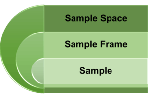
Types of sampling methods
Before we go into the specifics of each sampling method, it’s vital to understand terms like sample, sample frame, and sample space. In probability theory, the sample space comprises all possible outcomes of a random experiment, while the sample frame is the list or source guiding sample selection in statistical research. The sample represents the group of individuals participating in the study, forming the basis for the research findings. Selecting the correct sample is critical to ensuring the validity and reliability of any research; the sample should be representative of the population.
There are two most common sampling methods:
- Probability sampling: A sampling method in which each unit or element in the population has an equal chance of being selected in the final sample. This is called random sampling, emphasizing the random and non-zero probability nature of selecting samples. Such a sampling technique ensures a more representative and unbiased sample, enabling robust inferences about the entire population.
- Non-probability sampling: Another sampling method is non-probability sampling, which involves collecting data conveniently through a non-random selection based on predefined criteria. This offers a straightforward way to gather data, although the resulting sample may or may not accurately represent the entire population.
Irrespective of the research method you opt for, it is essential to explicitly state the chosen sampling technique in the methodology section of your research article. Now, we will explore the different characteristics of both sampling methods, along with various subtypes falling under these categories.
What is probability sampling?
The probability sampling method is based on the probability theory, which means that the sample selection criteria involve some random selection. The probability sampling method provides an equal opportunity for all elements or units within the entire sample space to be chosen. While it can be labor-intensive and expensive, the advantage lies in its ability to offer a more accurate representation of the population, thereby enhancing confidence in the inferences drawn in the research.
Types of probability sampling
Various probability sampling methods exist, such as simple random sampling, systematic sampling, stratified sampling, and clustered sampling. Here, we provide detailed discussions and illustrative examples for each of these sampling methods:

- Simple random sampling: In simple random sampling, each individual has an equal probability of being chosen, and each selection is independent of the others. Because the choice is entirely based on chance, this is also known as the method of chance selection. In the simple random sampling method, the sample frame comprises the entire population.
For example, A fitness sports brand is launching a new protein drink and aims to select 20 individuals from a 200-person fitness center to try it. Employing a simple random sampling approach, each of the 200 people is assigned a unique identifier. Of these, 20 individuals are then chosen by generating random numbers between 1 and 200, either manually or through a computer program. Matching these numbers with the individuals creates a randomly selected group of 20 people. This method minimizes sampling bias and ensures a representative subset of the entire population under study.

- Systematic sampling: The systematic sampling approach involves selecting units or elements at regular intervals from an ordered list of the population. Because the starting point of this sampling method is chosen at random, it is more convenient than essential random sampling. For a better understanding, consider the following example.
For example, considering the previous model, individuals at the fitness facility are arranged alphabetically. The manufacturer then initiates the process by randomly selecting a starting point from the first ten positions, let’s say 8. Starting from the 8th position, every tenth person on the list is then chosen (e.g., 8, 18, 28, 38, and so forth) until a sample of 20 individuals is obtained.

- Stratified sampling: Stratified sampling divides the population into subgroups (strata), and random samples are drawn from each stratum in proportion to its size in the population. Stratified sampling provides improved representation because each subgroup that differs in significant ways is included in the final sample.
For example, Expanding on the previous simple random sampling example, suppose the manufacturer aims for a more comprehensive representation of genders in a sample of 200 people, consisting of 90 males, 80 females, and 30 others. The manufacturer categorizes the population into three gender strata (Male, Female, and Others). Within each group, random sampling is employed to select nine males, eight females, and three individuals from the others category, resulting in a well-rounded and representative sample of 200 individuals.
- Clustered sampling: In this sampling method, the population is divided into clusters, and then a random sample of clusters is included in the final sample. Clustered sampling, distinct from stratified sampling, involves subgroups (clusters) that exhibit characteristics similar to the whole sample. In the case of small clusters, all members can be included in the final sample, whereas for larger clusters, individuals within each cluster may be sampled using the sampling above methods. This approach is referred to as multistage sampling. This sampling method is well-suited for large and widely distributed populations; however, there is a potential risk of sample error because ensuring that the sampled clusters truly represent the entire population can be challenging.

For example, Researchers conducting a nationwide health study can select specific geographic clusters, like cities or regions, instead of trying to survey the entire population individually. Within each chosen cluster, they sample individuals, providing a representative subset without the logistical challenges of attempting a nationwide survey.
Use s of probability sampling
Probability sampling methods find widespread use across diverse research disciplines because of their ability to yield representative and unbiased samples. The advantages of employing probability sampling include the following:
- Representativeness
Probability sampling assures that every element in the population has a non-zero chance of being included in the sample, ensuring representativeness of the entire population and decreasing research bias to minimal to non-existent levels. The researcher can acquire higher-quality data via probability sampling, increasing confidence in the conclusions.
- Statistical inference
Statistical methods, like confidence intervals and hypothesis testing, depend on probability sampling to generalize findings from a sample to the broader population. Probability sampling methods ensure unbiased representation, allowing inferences about the population based on the characteristics of the sample.
- Precision and reliability
The use of probability sampling improves the precision and reliability of study results. Because the probability of selecting any single element/individual is known, the chance variations that may occur in non-probability sampling methods are reduced, resulting in more dependable and precise estimations.
- Generalizability
Probability sampling enables the researcher to generalize study findings to the entire population from which they were derived. The results produced through probability sampling methods are more likely to be applicable to the larger population, laying the foundation for making broad predictions or recommendations.
- Minimization of Selection Bias
By ensuring that each member of the population has an equal chance of being selected in the sample, probability sampling lowers the possibility of selection bias. This reduces the impact of systematic errors that may occur in non-probability sampling methods, where data may be skewed toward a specific demographic due to inadequate representation of each segment of the population.
What is non-probability sampling?
Non-probability sampling methods involve selecting individuals based on non-random criteria, often relying on the researcher’s judgment or predefined criteria. While it is easier and more economical, it tends to introduce sampling bias, resulting in weaker inferences compared to probability sampling techniques in research.
Types of Non-probability Sampling
Non-probability sampling methods are further classified as convenience sampling, consecutive sampling, quota sampling, purposive or judgmental sampling, and snowball sampling. Let’s explore these types of sampling methods in detail.
- Convenience sampling: In convenience sampling, individuals are recruited directly from the population based on the accessibility and proximity to the researcher. It is a simple, inexpensive, and practical method of sample selection, yet convenience sampling suffers from both sampling and selection bias due to a lack of appropriate population representation.

For example, imagine you’re a researcher investigating smartphone usage patterns in your city. The most convenient way to select participants is by approaching people in a shopping mall on a weekday afternoon. However, this convenience sampling method may not be an accurate representation of the city’s overall smartphone usage patterns as the sample is limited to individuals present at the mall during weekdays, excluding those who visit on other days or never visit the mall.
- Consecutive sampling: Participants in consecutive sampling (or sequential sampling) are chosen based on their availability and desire to participate in the study as they become available. This strategy entails sequentially recruiting individuals who fulfill the researcher’s requirements.
For example, In researching the prevalence of stroke in a hospital, instead of randomly selecting patients from the entire population, the researcher can opt to include all eligible patients admitted over three months. Participants are then consecutively recruited upon admission during that timeframe, forming the study sample.
- Quota sampling: The selection of individuals in quota sampling is based on non-random selection criteria in which only participants with certain traits or proportions that are representative of the population are included. Quota sampling involves setting predetermined quotas for specific subgroups based on key demographics or other relevant characteristics. This sampling method employs dividing the population into mutually exclusive subgroups and then selecting sample units until the set quota is reached.

For example, In a survey on a college campus to assess student interest in a new policy, the researcher should establish quotas aligned with the distribution of student majors, ensuring representation from various academic disciplines. If the campus has 20% biology majors, 30% engineering majors, 20% business majors, and 30% liberal arts majors, participants should be recruited to mirror these proportions.
- Purposive or judgmental sampling: In purposive sampling, the researcher leverages expertise to select a sample relevant to the study’s specific questions. This sampling method is commonly applied in qualitative research, mainly when aiming to understand a particular phenomenon, and is suitable for smaller population sizes.

For example, imagine a researcher who wants to study public policy issues for a focus group. The researcher might purposely select participants with expertise in economics, law, and public administration to take advantage of their knowledge and ensure a depth of understanding.
- Snowball sampling: This sampling method is used when accessing the population is challenging. It involves collecting the sample through a chain-referral process, where each recruited candidate aids in finding others. These candidates share common traits, representing the targeted population. This method is often used in qualitative research, particularly when studying phenomena related to stigmatized or hidden populations.

For example, In a study focusing on understanding the experiences and challenges of individuals in hidden or stigmatized communities (e.g., LGBTQ+ individuals in specific cultural contexts), the snowball sampling technique can be employed. The researcher initiates contact with one community member, who then assists in identifying additional candidates until the desired sample size is achieved.
Uses of non-probability sampling
Non-probability sampling approaches are employed in qualitative or exploratory research where the goal is to investigate underlying population traits rather than generalizability. Non-probability sampling methods are also helpful for the following purposes:
- Generating a hypothesis
In the initial stages of exploratory research, non-probability methods such as purposive or convenience allow researchers to quickly gather information and generate hypothesis that helps build a future research plan.
- Qualitative research
Qualitative research is usually focused on understanding the depth and complexity of human experiences, behaviors, and perspectives. Non-probability methods like purposive or snowball sampling are commonly used to select participants with specific traits that are relevant to the research question.
- Convenience and pragmatism
Non-probability sampling methods are valuable when resource and time are limited or when preliminary data is required to test the pilot study. For example, conducting a survey at a local shopping mall to gather opinions on a consumer product due to the ease of access to potential participants.
Probability vs Non-probability Sampling Methods
| Selection of participants | Random selection of participants from the population using randomization methods | Non-random selection of participants from the population based on convenience or criteria |
| Representativeness | Likely to yield a representative sample of the whole population allowing for generalizations | May not yield a representative sample of the whole population; poor generalizability |
| Precision and accuracy | Provides more precise and accurate estimates of population characteristics | May have less precision and accuracy due to non-random selection |
| Bias | Minimizes selection bias | May introduce selection bias if criteria are subjective and not well-defined |
| Statistical inference | Suited for statistical inference and hypothesis testing and for making generalization to the population | Less suited for statistical inference and hypothesis testing on the population |
| Application | Useful for quantitative research where generalizability is crucial | Commonly used in qualitative and exploratory research where in-depth insights are the goal |
Frequently asked questions
- What is multistage sampling ? Multistage sampling is a form of probability sampling approach that involves the progressive selection of samples in stages, going from larger clusters to a small number of participants, making it suited for large-scale research with enormous population lists.
- What are the methods of probability sampling? Probability sampling methods are simple random sampling, stratified random sampling, systematic sampling, cluster sampling, and multistage sampling.
- How to decide which type of sampling method to use? Choose a sampling method based on the goals, population, and resources. Probability for statistics and non-probability for efficiency or qualitative insights can be considered . Also, consider the population characteristics, size, and alignment with study objectives.
- What are the methods of non-probability sampling? Non-probability sampling methods are convenience sampling, consecutive sampling, purposive sampling, snowball sampling, and quota sampling.
- Why are sampling methods used in research? Sampling methods in research are employed to efficiently gather representative data from a subset of a larger population, enabling valid conclusions and generalizations while minimizing costs and time.
R Discovery is a literature search and research reading platform that accelerates your research discovery journey by keeping you updated on the latest, most relevant scholarly content. With 250M+ research articles sourced from trusted aggregators like CrossRef, Unpaywall, PubMed, PubMed Central, Open Alex and top publishing houses like Springer Nature, JAMA, IOP, Taylor & Francis, NEJM, BMJ, Karger, SAGE, Emerald Publishing and more, R Discovery puts a world of research at your fingertips.
Try R Discovery Prime FREE for 1 week or upgrade at just US$72 a year to access premium features that let you listen to research on the go, read in your language, collaborate with peers, auto sync with reference managers, and much more. Choose a simpler, smarter way to find and read research – Download the app and start your free 7-day trial today !
Related Posts

Research in Shorts: R Discovery’s New Feature Helps Academics Assess Relevant Papers in 2mins

Research Paper Appendix: Format and Examples
Sampling Methods & Strategies 101
Everything you need to know (including examples)
By: Derek Jansen (MBA) | Expert Reviewed By: Kerryn Warren (PhD) | January 2023
If you’re new to research, sooner or later you’re bound to wander into the intimidating world of sampling methods and strategies. If you find yourself on this page, chances are you’re feeling a little overwhelmed or confused. Fear not – in this post we’ll unpack sampling in straightforward language , along with loads of examples .
Overview: Sampling Methods & Strategies
- What is sampling in a research context?
- The two overarching approaches
Simple random sampling
Stratified random sampling, cluster sampling, systematic sampling, purposive sampling, convenience sampling, snowball sampling.
- How to choose the right sampling method
What (exactly) is sampling?
At the simplest level, sampling (within a research context) is the process of selecting a subset of participants from a larger group . For example, if your research involved assessing US consumers’ perceptions about a particular brand of laundry detergent, you wouldn’t be able to collect data from every single person that uses laundry detergent (good luck with that!) – but you could potentially collect data from a smaller subset of this group.
In technical terms, the larger group is referred to as the population , and the subset (the group you’ll actually engage with in your research) is called the sample . Put another way, you can look at the population as a full cake and the sample as a single slice of that cake. In an ideal world, you’d want your sample to be perfectly representative of the population, as that would allow you to generalise your findings to the entire population. In other words, you’d want to cut a perfect cross-sectional slice of cake, such that the slice reflects every layer of the cake in perfect proportion.
Achieving a truly representative sample is, unfortunately, a little trickier than slicing a cake, as there are many practical challenges and obstacles to achieving this in a real-world setting. Thankfully though, you don’t always need to have a perfectly representative sample – it all depends on the specific research aims of each study – so don’t stress yourself out about that just yet!
With the concept of sampling broadly defined, let’s look at the different approaches to sampling to get a better understanding of what it all looks like in practice.

The two overarching sampling approaches
At the highest level, there are two approaches to sampling: probability sampling and non-probability sampling . Within each of these, there are a variety of sampling methods , which we’ll explore a little later.
Probability sampling involves selecting participants (or any unit of interest) on a statistically random basis , which is why it’s also called “random sampling”. In other words, the selection of each individual participant is based on a pre-determined process (not the discretion of the researcher). As a result, this approach achieves a random sample.
Probability-based sampling methods are most commonly used in quantitative research , especially when it’s important to achieve a representative sample that allows the researcher to generalise their findings.
Non-probability sampling , on the other hand, refers to sampling methods in which the selection of participants is not statistically random . In other words, the selection of individual participants is based on the discretion and judgment of the researcher, rather than on a pre-determined process.
Non-probability sampling methods are commonly used in qualitative research , where the richness and depth of the data are more important than the generalisability of the findings.
If that all sounds a little too conceptual and fluffy, don’t worry. Let’s take a look at some actual sampling methods to make it more tangible.
Need a helping hand?
Probability-based sampling methods
First, we’ll look at four common probability-based (random) sampling methods:
Importantly, this is not a comprehensive list of all the probability sampling methods – these are just four of the most common ones. So, if you’re interested in adopting a probability-based sampling approach, be sure to explore all the options.
Simple random sampling involves selecting participants in a completely random fashion , where each participant has an equal chance of being selected. Basically, this sampling method is the equivalent of pulling names out of a hat , except that you can do it digitally. For example, if you had a list of 500 people, you could use a random number generator to draw a list of 50 numbers (each number, reflecting a participant) and then use that dataset as your sample.
Thanks to its simplicity, simple random sampling is easy to implement , and as a consequence, is typically quite cheap and efficient . Given that the selection process is completely random, the results can be generalised fairly reliably. However, this also means it can hide the impact of large subgroups within the data, which can result in minority subgroups having little representation in the results – if any at all. To address this, one needs to take a slightly different approach, which we’ll look at next.
Stratified random sampling is similar to simple random sampling, but it kicks things up a notch. As the name suggests, stratified sampling involves selecting participants randomly , but from within certain pre-defined subgroups (i.e., strata) that share a common trait . For example, you might divide the population into strata based on gender, ethnicity, age range or level of education, and then select randomly from each group.
The benefit of this sampling method is that it gives you more control over the impact of large subgroups (strata) within the population. For example, if a population comprises 80% males and 20% females, you may want to “balance” this skew out by selecting a random sample from an equal number of males and females. This would, of course, reduce the representativeness of the sample, but it would allow you to identify differences between subgroups. So, depending on your research aims, the stratified approach could work well.

Next on the list is cluster sampling. As the name suggests, this sampling method involves sampling from naturally occurring, mutually exclusive clusters within a population – for example, area codes within a city or cities within a country. Once the clusters are defined, a set of clusters are randomly selected and then a set of participants are randomly selected from each cluster.
Now, you’re probably wondering, “how is cluster sampling different from stratified random sampling?”. Well, let’s look at the previous example where each cluster reflects an area code in a given city.
With cluster sampling, you would collect data from clusters of participants in a handful of area codes (let’s say 5 neighbourhoods). Conversely, with stratified random sampling, you would need to collect data from all over the city (i.e., many more neighbourhoods). You’d still achieve the same sample size either way (let’s say 200 people, for example), but with stratified sampling, you’d need to do a lot more running around, as participants would be scattered across a vast geographic area. As a result, cluster sampling is often the more practical and economical option.
If that all sounds a little mind-bending, you can use the following general rule of thumb. If a population is relatively homogeneous , cluster sampling will often be adequate. Conversely, if a population is quite heterogeneous (i.e., diverse), stratified sampling will generally be more appropriate.
The last probability sampling method we’ll look at is systematic sampling. This method simply involves selecting participants at a set interval , starting from a random point .
For example, if you have a list of students that reflects the population of a university, you could systematically sample that population by selecting participants at an interval of 8 . In other words, you would randomly select a starting point – let’s say student number 40 – followed by student 48, 56, 64, etc.
What’s important with systematic sampling is that the population list you select from needs to be randomly ordered . If there are underlying patterns in the list (for example, if the list is ordered by gender, IQ, age, etc.), this will result in a non-random sample, which would defeat the purpose of adopting this sampling method. Of course, you could safeguard against this by “shuffling” your population list using a random number generator or similar tool.

Non-probability-based sampling methods
Right, now that we’ve looked at a few probability-based sampling methods, let’s look at three non-probability methods :
Again, this is not an exhaustive list of all possible sampling methods, so be sure to explore further if you’re interested in adopting a non-probability sampling approach.
First up, we’ve got purposive sampling – also known as judgment , selective or subjective sampling. Again, the name provides some clues, as this method involves the researcher selecting participants using his or her own judgement , based on the purpose of the study (i.e., the research aims).
For example, suppose your research aims were to understand the perceptions of hyper-loyal customers of a particular retail store. In that case, you could use your judgement to engage with frequent shoppers, as well as rare or occasional shoppers, to understand what judgements drive the two behavioural extremes .
Purposive sampling is often used in studies where the aim is to gather information from a small population (especially rare or hard-to-find populations), as it allows the researcher to target specific individuals who have unique knowledge or experience . Naturally, this sampling method is quite prone to researcher bias and judgement error, and it’s unlikely to produce generalisable results, so it’s best suited to studies where the aim is to go deep rather than broad .

Next up, we have convenience sampling. As the name suggests, with this method, participants are selected based on their availability or accessibility . In other words, the sample is selected based on how convenient it is for the researcher to access it, as opposed to using a defined and objective process.
Naturally, convenience sampling provides a quick and easy way to gather data, as the sample is selected based on the individuals who are readily available or willing to participate. This makes it an attractive option if you’re particularly tight on resources and/or time. However, as you’d expect, this sampling method is unlikely to produce a representative sample and will of course be vulnerable to researcher bias , so it’s important to approach it with caution.
Last but not least, we have the snowball sampling method. This method relies on referrals from initial participants to recruit additional participants. In other words, the initial subjects form the first (small) snowball and each additional subject recruited through referral is added to the snowball, making it larger as it rolls along .
Snowball sampling is often used in research contexts where it’s difficult to identify and access a particular population. For example, people with a rare medical condition or members of an exclusive group. It can also be useful in cases where the research topic is sensitive or taboo and people are unlikely to open up unless they’re referred by someone they trust.
Simply put, snowball sampling is ideal for research that involves reaching hard-to-access populations . But, keep in mind that, once again, it’s a sampling method that’s highly prone to researcher bias and is unlikely to produce a representative sample. So, make sure that it aligns with your research aims and questions before adopting this method.
How to choose a sampling method
Now that we’ve looked at a few popular sampling methods (both probability and non-probability based), the obvious question is, “ how do I choose the right sampling method for my study?”. When selecting a sampling method for your research project, you’ll need to consider two important factors: your research aims and your resources .
As with all research design and methodology choices, your sampling approach needs to be guided by and aligned with your research aims, objectives and research questions – in other words, your golden thread. Specifically, you need to consider whether your research aims are primarily concerned with producing generalisable findings (in which case, you’ll likely opt for a probability-based sampling method) or with achieving rich , deep insights (in which case, a non-probability-based approach could be more practical). Typically, quantitative studies lean toward the former, while qualitative studies aim for the latter, so be sure to consider your broader methodology as well.
The second factor you need to consider is your resources and, more generally, the practical constraints at play. If, for example, you have easy, free access to a large sample at your workplace or university and a healthy budget to help you attract participants, that will open up multiple options in terms of sampling methods. Conversely, if you’re cash-strapped, short on time and don’t have unfettered access to your population of interest, you may be restricted to convenience or referral-based methods.
In short, be ready for trade-offs – you won’t always be able to utilise the “perfect” sampling method for your study, and that’s okay. Much like all the other methodological choices you’ll make as part of your study, you’ll often need to compromise and accept practical trade-offs when it comes to sampling. Don’t let this get you down though – as long as your sampling choice is well explained and justified, and the limitations of your approach are clearly articulated, you’ll be on the right track.

Let’s recap…
In this post, we’ve covered the basics of sampling within the context of a typical research project.
- Sampling refers to the process of defining a subgroup (sample) from the larger group of interest (population).
- The two overarching approaches to sampling are probability sampling (random) and non-probability sampling .
- Common probability-based sampling methods include simple random sampling, stratified random sampling, cluster sampling and systematic sampling.
- Common non-probability-based sampling methods include purposive sampling, convenience sampling and snowball sampling.
- When choosing a sampling method, you need to consider your research aims , objectives and questions, as well as your resources and other practical constraints .
If you’d like to see an example of a sampling strategy in action, be sure to check out our research methodology chapter sample .
Last but not least, if you need hands-on help with your sampling (or any other aspect of your research), take a look at our 1-on-1 coaching service , where we guide you through each step of the research process, at your own pace.

Psst... there’s more!
This post was based on one of our popular Research Bootcamps . If you're working on a research project, you'll definitely want to check this out ...

Excellent and helpful. Best site to get a full understanding of Research methodology. I’m nolonger as “clueless “..😉

Excellent and helpful for junior researcher!

Grad Coach tutorials are excellent – I recommend them to everyone doing research. I will be working with a sample of imprisoned women and now have a much clearer idea concerning sampling. Thank you to all at Grad Coach for generously sharing your expertise with students.
Submit a Comment Cancel reply
Your email address will not be published. Required fields are marked *
Save my name, email, and website in this browser for the next time I comment.
- Print Friendly
Sampling Methods In Reseach: Types, Techniques, & Examples
Saul McLeod, PhD
Editor-in-Chief for Simply Psychology
BSc (Hons) Psychology, MRes, PhD, University of Manchester
Saul McLeod, PhD., is a qualified psychology teacher with over 18 years of experience in further and higher education. He has been published in peer-reviewed journals, including the Journal of Clinical Psychology.
Learn about our Editorial Process
Olivia Guy-Evans, MSc
Associate Editor for Simply Psychology
BSc (Hons) Psychology, MSc Psychology of Education
Olivia Guy-Evans is a writer and associate editor for Simply Psychology. She has previously worked in healthcare and educational sectors.
On This Page:
Sampling methods in psychology refer to strategies used to select a subset of individuals (a sample) from a larger population, to study and draw inferences about the entire population. Common methods include random sampling, stratified sampling, cluster sampling, and convenience sampling. Proper sampling ensures representative, generalizable, and valid research results.
- Sampling : the process of selecting a representative group from the population under study.
- Target population : the total group of individuals from which the sample might be drawn.
- Sample: a subset of individuals selected from a larger population for study or investigation. Those included in the sample are termed “participants.”
- Generalizability : the ability to apply research findings from a sample to the broader target population, contingent on the sample being representative of that population.
For instance, if the advert for volunteers is published in the New York Times, this limits how much the study’s findings can be generalized to the whole population, because NYT readers may not represent the entire population in certain respects (e.g., politically, socio-economically).
The Purpose of Sampling
We are interested in learning about large groups of people with something in common in psychological research. We call the group interested in studying our “target population.”
In some types of research, the target population might be as broad as all humans. Still, in other types of research, the target population might be a smaller group, such as teenagers, preschool children, or people who misuse drugs.

Studying every person in a target population is more or less impossible. Hence, psychologists select a sample or sub-group of the population that is likely to be representative of the target population we are interested in.
This is important because we want to generalize from the sample to the target population. The more representative the sample, the more confident the researcher can be that the results can be generalized to the target population.
One of the problems that can occur when selecting a sample from a target population is sampling bias. Sampling bias refers to situations where the sample does not reflect the characteristics of the target population.
Many psychology studies have a biased sample because they have used an opportunity sample that comprises university students as their participants (e.g., Asch ).
OK, so you’ve thought up this brilliant psychological study and designed it perfectly. But who will you try it out on, and how will you select your participants?
There are various sampling methods. The one chosen will depend on a number of factors (such as time, money, etc.).

Random Sampling
Random sampling is a type of probability sampling where everyone in the entire target population has an equal chance of being selected.
This is similar to the national lottery. If the “population” is everyone who bought a lottery ticket, then everyone has an equal chance of winning the lottery (assuming they all have one ticket each).
Random samples require naming or numbering the target population and then using some raffle method to choose those to make up the sample. Random samples are the best method of selecting your sample from the population of interest.
- The advantages are that your sample should represent the target population and eliminate sampling bias.
- The disadvantage is that it is very difficult to achieve (i.e., time, effort, and money).
Stratified Sampling
During stratified sampling , the researcher identifies the different types of people that make up the target population and works out the proportions needed for the sample to be representative.
A list is made of each variable (e.g., IQ, gender, etc.) that might have an effect on the research. For example, if we are interested in the money spent on books by undergraduates, then the main subject studied may be an important variable.
For example, students studying English Literature may spend more money on books than engineering students, so if we use a large percentage of English students or engineering students, our results will not be accurate.
We have to determine the relative percentage of each group at a university, e.g., Engineering 10%, Social Sciences 15%, English 20%, Sciences 25%, Languages 10%, Law 5%, and Medicine 15%. The sample must then contain all these groups in the same proportion as the target population (university students).
- The disadvantage of stratified sampling is that gathering such a sample would be extremely time-consuming and difficult to do. This method is rarely used in Psychology.
- However, the advantage is that the sample should be highly representative of the target population, and therefore we can generalize from the results obtained.
Opportunity Sampling
Opportunity sampling is a method in which participants are chosen based on their ease of availability and proximity to the researcher, rather than using random or systematic criteria. It’s a type of convenience sampling .
An opportunity sample is obtained by asking members of the population of interest if they would participate in your research. An example would be selecting a sample of students from those coming out of the library.
- This is a quick and easy way of choosing participants (advantage)
- It may not provide a representative sample and could be biased (disadvantage).
Systematic Sampling
Systematic sampling is a method where every nth individual is selected from a list or sequence to form a sample, ensuring even and regular intervals between chosen subjects.
Participants are systematically selected (i.e., orderly/logical) from the target population, like every nth participant on a list of names.
To take a systematic sample, you list all the population members and then decide upon a sample you would like. By dividing the number of people in the population by the number of people you want in your sample, you get a number we will call n.
If you take every nth name, you will get a systematic sample of the correct size. If, for example, you wanted to sample 150 children from a school of 1,500, you would take every 10th name.
- The advantage of this method is that it should provide a representative sample.
Sample size
The sample size is a critical factor in determining the reliability and validity of a study’s findings. While increasing the sample size can enhance the generalizability of results, it’s also essential to balance practical considerations, such as resource constraints and diminishing returns from ever-larger samples.
Reliability and Validity
Reliability refers to the consistency and reproducibility of research findings across different occasions, researchers, or instruments. A small sample size may lead to inconsistent results due to increased susceptibility to random error or the influence of outliers. In contrast, a larger sample minimizes these errors, promoting more reliable results.
Validity pertains to the accuracy and truthfulness of research findings. For a study to be valid, it should accurately measure what it intends to do. A small, unrepresentative sample can compromise external validity, meaning the results don’t generalize well to the larger population. A larger sample captures more variability, ensuring that specific subgroups or anomalies don’t overly influence results.
Practical Considerations
Resource Constraints : Larger samples demand more time, money, and resources. Data collection becomes more extensive, data analysis more complex, and logistics more challenging.
Diminishing Returns : While increasing the sample size generally leads to improved accuracy and precision, there’s a point where adding more participants yields only marginal benefits. For instance, going from 50 to 500 participants might significantly boost a study’s robustness, but jumping from 10,000 to 10,500 might not offer a comparable advantage, especially considering the added costs.
- Privacy Policy
Home » Sampling Methods – Types, Techniques and Examples
Sampling Methods – Types, Techniques and Examples
Table of Contents

Sampling refers to the process of selecting a subset of data from a larger population or dataset in order to analyze or make inferences about the whole population.
In other words, sampling involves taking a representative sample of data from a larger group or dataset in order to gain insights or draw conclusions about the entire group.
Sampling Methods
Sampling methods refer to the techniques used to select a subset of individuals or units from a larger population for the purpose of conducting statistical analysis or research.
Sampling is an essential part of the Research because it allows researchers to draw conclusions about a population without having to collect data from every member of that population, which can be time-consuming, expensive, or even impossible.
Types of Sampling Methods
Sampling can be broadly categorized into two main categories:
Probability Sampling
This type of sampling is based on the principles of random selection, and it involves selecting samples in a way that every member of the population has an equal chance of being included in the sample.. Probability sampling is commonly used in scientific research and statistical analysis, as it provides a representative sample that can be generalized to the larger population.
Type of Probability Sampling :
- Simple Random Sampling: In this method, every member of the population has an equal chance of being selected for the sample. This can be done using a random number generator or by drawing names out of a hat, for example.
- Systematic Sampling: In this method, the population is first divided into a list or sequence, and then every nth member is selected for the sample. For example, if every 10th person is selected from a list of 100 people, the sample would include 10 people.
- Stratified Sampling: In this method, the population is divided into subgroups or strata based on certain characteristics, and then a random sample is taken from each stratum. This is often used to ensure that the sample is representative of the population as a whole.
- Cluster Sampling: In this method, the population is divided into clusters or groups, and then a random sample of clusters is selected. Then, all members of the selected clusters are included in the sample.
- Multi-Stage Sampling : This method combines two or more sampling techniques. For example, a researcher may use stratified sampling to select clusters, and then use simple random sampling to select members within each cluster.
Non-probability Sampling
This type of sampling does not rely on random selection, and it involves selecting samples in a way that does not give every member of the population an equal chance of being included in the sample. Non-probability sampling is often used in qualitative research, where the aim is not to generalize findings to a larger population, but to gain an in-depth understanding of a particular phenomenon or group. Non-probability sampling methods can be quicker and more cost-effective than probability sampling methods, but they may also be subject to bias and may not be representative of the larger population.
Types of Non-probability Sampling :
- Convenience Sampling: In this method, participants are chosen based on their availability or willingness to participate. This method is easy and convenient but may not be representative of the population.
- Purposive Sampling: In this method, participants are selected based on specific criteria, such as their expertise or knowledge on a particular topic. This method is often used in qualitative research, but may not be representative of the population.
- Snowball Sampling: In this method, participants are recruited through referrals from other participants. This method is often used when the population is hard to reach, but may not be representative of the population.
- Quota Sampling: In this method, a predetermined number of participants are selected based on specific criteria, such as age or gender. This method is often used in market research, but may not be representative of the population.
- Volunteer Sampling: In this method, participants volunteer to participate in the study. This method is often used in research where participants are motivated by personal interest or altruism, but may not be representative of the population.
Applications of Sampling Methods
Applications of Sampling Methods from different fields:
- Psychology : Sampling methods are used in psychology research to study various aspects of human behavior and mental processes. For example, researchers may use stratified sampling to select a sample of participants that is representative of the population based on factors such as age, gender, and ethnicity. Random sampling may also be used to select participants for experimental studies.
- Sociology : Sampling methods are commonly used in sociological research to study social phenomena and relationships between individuals and groups. For example, researchers may use cluster sampling to select a sample of neighborhoods to study the effects of economic inequality on health outcomes. Stratified sampling may also be used to select a sample of participants that is representative of the population based on factors such as income, education, and occupation.
- Social sciences: Sampling methods are commonly used in social sciences to study human behavior and attitudes. For example, researchers may use stratified sampling to select a sample of participants that is representative of the population based on factors such as age, gender, and income.
- Marketing : Sampling methods are used in marketing research to collect data on consumer preferences, behavior, and attitudes. For example, researchers may use random sampling to select a sample of consumers to participate in a survey about a new product.
- Healthcare : Sampling methods are used in healthcare research to study the prevalence of diseases and risk factors, and to evaluate interventions. For example, researchers may use cluster sampling to select a sample of health clinics to participate in a study of the effectiveness of a new treatment.
- Environmental science: Sampling methods are used in environmental science to collect data on environmental variables such as water quality, air pollution, and soil composition. For example, researchers may use systematic sampling to collect soil samples at regular intervals across a field.
- Education : Sampling methods are used in education research to study student learning and achievement. For example, researchers may use stratified sampling to select a sample of schools that is representative of the population based on factors such as demographics and academic performance.
Examples of Sampling Methods
Probability Sampling Methods Examples:
- Simple random sampling Example : A researcher randomly selects participants from the population using a random number generator or drawing names from a hat.
- Stratified random sampling Example : A researcher divides the population into subgroups (strata) based on a characteristic of interest (e.g. age or income) and then randomly selects participants from each subgroup.
- Systematic sampling Example : A researcher selects participants at regular intervals from a list of the population.
Non-probability Sampling Methods Examples:
- Convenience sampling Example: A researcher selects participants who are conveniently available, such as students in a particular class or visitors to a shopping mall.
- Purposive sampling Example : A researcher selects participants who meet specific criteria, such as individuals who have been diagnosed with a particular medical condition.
- Snowball sampling Example : A researcher selects participants who are referred to them by other participants, such as friends or acquaintances.
How to Conduct Sampling Methods
some general steps to conduct sampling methods:
- Define the population: Identify the population of interest and clearly define its boundaries.
- Choose the sampling method: Select an appropriate sampling method based on the research question, characteristics of the population, and available resources.
- Determine the sample size: Determine the desired sample size based on statistical considerations such as margin of error, confidence level, or power analysis.
- Create a sampling frame: Develop a list of all individuals or elements in the population from which the sample will be drawn. The sampling frame should be comprehensive, accurate, and up-to-date.
- Select the sample: Use the chosen sampling method to select the sample from the sampling frame. The sample should be selected randomly, or if using a non-random method, every effort should be made to minimize bias and ensure that the sample is representative of the population.
- Collect data: Once the sample has been selected, collect data from each member of the sample using appropriate research methods (e.g., surveys, interviews, observations).
- Analyze the data: Analyze the data collected from the sample to draw conclusions about the population of interest.
When to use Sampling Methods
Sampling methods are used in research when it is not feasible or practical to study the entire population of interest. Sampling allows researchers to study a smaller group of individuals, known as a sample, and use the findings from the sample to make inferences about the larger population.
Sampling methods are particularly useful when:
- The population of interest is too large to study in its entirety.
- The cost and time required to study the entire population are prohibitive.
- The population is geographically dispersed or difficult to access.
- The research question requires specialized or hard-to-find individuals.
- The data collected is quantitative and statistical analyses are used to draw conclusions.
Purpose of Sampling Methods
The main purpose of sampling methods in research is to obtain a representative sample of individuals or elements from a larger population of interest, in order to make inferences about the population as a whole. By studying a smaller group of individuals, known as a sample, researchers can gather information about the population that would be difficult or impossible to obtain from studying the entire population.
Sampling methods allow researchers to:
- Study a smaller, more manageable group of individuals, which is typically less time-consuming and less expensive than studying the entire population.
- Reduce the potential for data collection errors and improve the accuracy of the results by minimizing sampling bias.
- Make inferences about the larger population with a certain degree of confidence, using statistical analyses of the data collected from the sample.
- Improve the generalizability and external validity of the findings by ensuring that the sample is representative of the population of interest.
Characteristics of Sampling Methods
Here are some characteristics of sampling methods:
- Randomness : Probability sampling methods are based on random selection, meaning that every member of the population has an equal chance of being selected. This helps to minimize bias and ensure that the sample is representative of the population.
- Representativeness : The goal of sampling is to obtain a sample that is representative of the larger population of interest. This means that the sample should reflect the characteristics of the population in terms of key demographic, behavioral, or other relevant variables.
- Size : The size of the sample should be large enough to provide sufficient statistical power for the research question at hand. The sample size should also be appropriate for the chosen sampling method and the level of precision desired.
- Efficiency : Sampling methods should be efficient in terms of time, cost, and resources required. The method chosen should be feasible given the available resources and time constraints.
- Bias : Sampling methods should aim to minimize bias and ensure that the sample is representative of the population of interest. Bias can be introduced through non-random selection or non-response, and can affect the validity and generalizability of the findings.
- Precision : Sampling methods should be precise in terms of providing estimates of the population parameters of interest. Precision is influenced by sample size, sampling method, and level of variability in the population.
- Validity : The validity of the sampling method is important for ensuring that the results obtained from the sample are accurate and can be generalized to the population of interest. Validity can be affected by sampling method, sample size, and the representativeness of the sample.
Advantages of Sampling Methods
Sampling methods have several advantages, including:
- Cost-Effective : Sampling methods are often much cheaper and less time-consuming than studying an entire population. By studying only a small subset of the population, researchers can gather valuable data without incurring the costs associated with studying the entire population.
- Convenience : Sampling methods are often more convenient than studying an entire population. For example, if a researcher wants to study the eating habits of people in a city, it would be very difficult and time-consuming to study every single person in the city. By using sampling methods, the researcher can obtain data from a smaller subset of people, making the study more feasible.
- Accuracy: When done correctly, sampling methods can be very accurate. By using appropriate sampling techniques, researchers can obtain a sample that is representative of the entire population. This allows them to make accurate generalizations about the population as a whole based on the data collected from the sample.
- Time-Saving: Sampling methods can save a lot of time compared to studying the entire population. By studying a smaller sample, researchers can collect data much more quickly than they could if they studied every single person in the population.
- Less Bias : Sampling methods can reduce bias in a study. If a researcher were to study the entire population, it would be very difficult to eliminate all sources of bias. However, by using appropriate sampling techniques, researchers can reduce bias and obtain a sample that is more representative of the entire population.
Limitations of Sampling Methods
- Sampling Error : Sampling error is the difference between the sample statistic and the population parameter. It is the result of selecting a sample rather than the entire population. The larger the sample, the lower the sampling error. However, no matter how large the sample size, there will always be some degree of sampling error.
- Selection Bias: Selection bias occurs when the sample is not representative of the population. This can happen if the sample is not selected randomly or if some groups are underrepresented in the sample. Selection bias can lead to inaccurate conclusions about the population.
- Non-response Bias : Non-response bias occurs when some members of the sample do not respond to the survey or study. This can result in a biased sample if the non-respondents differ from the respondents in important ways.
- Time and Cost : While sampling can be cost-effective, it can still be expensive and time-consuming to select a sample that is representative of the population. Depending on the sampling method used, it may take a long time to obtain a sample that is large enough and representative enough to be useful.
- Limited Information : Sampling can only provide information about the variables that are measured. It may not provide information about other variables that are relevant to the research question but were not measured.
- Generalization : The extent to which the findings from a sample can be generalized to the population depends on the representativeness of the sample. If the sample is not representative of the population, it may not be possible to generalize the findings to the population as a whole.
About the author

Muhammad Hassan
Researcher, Academic Writer, Web developer
You may also like

Convenience Sampling – Method, Types and Examples

Stratified Random Sampling – Definition, Method...

Purposive Sampling – Methods, Types and Examples

Snowball Sampling – Method, Types and Examples

Cluster Sampling – Types, Method and Examples

Simple Random Sampling – Types, Method and...
- En español – ExME
- Em português – EME
What are sampling methods and how do you choose the best one?
Posted on 18th November 2020 by Mohamed Khalifa

This tutorial will introduce sampling methods and potential sampling errors to avoid when conducting medical research.
Introduction to sampling methods
Examples of different sampling methods, choosing the best sampling method.
It is important to understand why we sample the population; for example, studies are built to investigate the relationships between risk factors and disease. In other words, we want to find out if this is a true association, while still aiming for the minimum risk for errors such as: chance, bias or confounding .
However, it would not be feasible to experiment on the whole population, we would need to take a good sample and aim to reduce the risk of having errors by proper sampling technique.
What is a sampling frame?
A sampling frame is a record of the target population containing all participants of interest. In other words, it is a list from which we can extract a sample.
What makes a good sample?
A good sample should be a representative subset of the population we are interested in studying, therefore, with each participant having equal chance of being randomly selected into the study.
We could choose a sampling method based on whether we want to account for sampling bias; a random sampling method is often preferred over a non-random method for this reason. Random sampling examples include: simple, systematic, stratified, and cluster sampling. Non-random sampling methods are liable to bias, and common examples include: convenience, purposive, snowballing, and quota sampling. For the purposes of this blog we will be focusing on random sampling methods .
Example: We want to conduct an experimental trial in a small population such as: employees in a company, or students in a college. We include everyone in a list and use a random number generator to select the participants
Advantages: Generalisable results possible, random sampling, the sampling frame is the whole population, every participant has an equal probability of being selected
Disadvantages: Less precise than stratified method, less representative than the systematic method

Example: Every nth patient entering the out-patient clinic is selected and included in our sample
Advantages: More feasible than simple or stratified methods, sampling frame is not always required
Disadvantages: Generalisability may decrease if baseline characteristics repeat across every nth participant

Example: We have a big population (a city) and we want to ensure representativeness of all groups with a pre-determined characteristic such as: age groups, ethnic origin, and gender
Advantages: Inclusive of strata (subgroups), reliable and generalisable results
Disadvantages: Does not work well with multiple variables

Example: 10 schools have the same number of students across the county. We can randomly select 3 out of 10 schools as our clusters
Advantages: Readily doable with most budgets, does not require a sampling frame
Disadvantages: Results may not be reliable nor generalisable

How can you identify sampling errors?
Non-random selection increases the probability of sampling (selection) bias if the sample does not represent the population we want to study. We could avoid this by random sampling and ensuring representativeness of our sample with regards to sample size.
An inadequate sample size decreases the confidence in our results as we may think there is no significant difference when actually there is. This type two error results from having a small sample size, or from participants dropping out of the sample.
In medical research of disease, if we select people with certain diseases while strictly excluding participants with other co-morbidities, we run the risk of diagnostic purity bias where important sub-groups of the population are not represented.
Furthermore, measurement bias may occur during re-collection of risk factors by participants (recall bias) or assessment of outcome where people who live longer are associated with treatment success, when in fact people who died were not included in the sample or data analysis (survivors bias).
By following the steps below we could choose the best sampling method for our study in an orderly fashion.
Research objectiveness
Firstly, a refined research question and goal would help us define our population of interest. If our calculated sample size is small then it would be easier to get a random sample. If, however, the sample size is large, then we should check if our budget and resources can handle a random sampling method.
Sampling frame availability
Secondly, we need to check for availability of a sampling frame (Simple), if not, could we make a list of our own (Stratified). If neither option is possible, we could still use other random sampling methods, for instance, systematic or cluster sampling.
Study design
Moreover, we could consider the prevalence of the topic (exposure or outcome) in the population, and what would be the suitable study design. In addition, checking if our target population is widely varied in its baseline characteristics. For example, a population with large ethnic subgroups could best be studied using a stratified sampling method.
Random sampling
Finally, the best sampling method is always the one that could best answer our research question while also allowing for others to make use of our results (generalisability of results). When we cannot afford a random sampling method, we can always choose from the non-random sampling methods.
To sum up, we now understand that choosing between random or non-random sampling methods is multifactorial. We might often be tempted to choose a convenience sample from the start, but that would not only decrease precision of our results, and would make us miss out on producing research that is more robust and reliable.
References (pdf)

Mohamed Khalifa
Leave a reply cancel reply.
Your email address will not be published. Required fields are marked *
Save my name, email, and website in this browser for the next time I comment.
No Comments on What are sampling methods and how do you choose the best one?

Thank you for this overview. A concise approach for research.

really helps! am an ecology student preparing to write my lab report for sampling.

I learned a lot to the given presentation.. It’s very comprehensive… Thanks for sharing…

Very informative and useful for my study. Thank you

Oversimplified info on sampling methods. Probabilistic of the sampling and sampling of samples by chance does rest solely on the random methods. Factors such as the random visits or presentation of the potential participants at clinics or sites could be sufficiently random in nature and should be used for the sake of efficiency and feasibility. Nevertheless, this approach has to be taken only after careful thoughts. Representativeness of the study samples have to be checked at the end or during reporting by comparing it to the published larger studies or register of some kind in/from the local population.

Thank you so much Mr.mohamed very useful and informative article
Subscribe to our newsletter
You will receive our monthly newsletter and free access to Trip Premium.
Related Articles

How to read a funnel plot
This blog introduces you to funnel plots, guiding you through how to read them and what may cause them to look asymmetrical.

Internal and external validity: what are they and how do they differ?
Is this study valid? Can I trust this study’s methods and design? Can I apply the results of this study to other contexts? Learn more about internal and external validity in research to help you answer these questions when you next look at a paper.

Cluster Randomized Trials: Concepts
This blog summarizes the concepts of cluster randomization, and the logistical and statistical considerations while designing a cluster randomized controlled trial.
Have a language expert improve your writing
Run a free plagiarism check in 10 minutes, automatically generate references for free.
- Knowledge Base
- Methodology
- Sampling Methods | Types, Techniques, & Examples
Sampling Methods | Types, Techniques, & Examples
Published on 3 May 2022 by Shona McCombes . Revised on 10 October 2022.
When you conduct research about a group of people, it’s rarely possible to collect data from every person in that group. Instead, you select a sample. The sample is the group of individuals who will actually participate in the research.
To draw valid conclusions from your results, you have to carefully decide how you will select a sample that is representative of the group as a whole. There are two types of sampling methods:
- Probability sampling involves random selection, allowing you to make strong statistical inferences about the whole group. It minimises the risk of selection bias .
- Non-probability sampling involves non-random selection based on convenience or other criteria, allowing you to easily collect data.
You should clearly explain how you selected your sample in the methodology section of your paper or thesis.
Table of contents
Population vs sample, probability sampling methods, non-probability sampling methods, frequently asked questions about sampling.
First, you need to understand the difference between a population and a sample , and identify the target population of your research.
- The population is the entire group that you want to draw conclusions about.
- The sample is the specific group of individuals that you will collect data from.
The population can be defined in terms of geographical location, age, income, and many other characteristics.

It is important to carefully define your target population according to the purpose and practicalities of your project.
If the population is very large, demographically mixed, and geographically dispersed, it might be difficult to gain access to a representative sample.
Sampling frame
The sampling frame is the actual list of individuals that the sample will be drawn from. Ideally, it should include the entire target population (and nobody who is not part of that population).
You are doing research on working conditions at Company X. Your population is all 1,000 employees of the company. Your sampling frame is the company’s HR database, which lists the names and contact details of every employee.
Sample size
The number of individuals you should include in your sample depends on various factors, including the size and variability of the population and your research design. There are different sample size calculators and formulas depending on what you want to achieve with statistical analysis .
Prevent plagiarism, run a free check.
Probability sampling means that every member of the population has a chance of being selected. It is mainly used in quantitative research . If you want to produce results that are representative of the whole population, probability sampling techniques are the most valid choice.
There are four main types of probability sample.

1. Simple random sampling
In a simple random sample , every member of the population has an equal chance of being selected. Your sampling frame should include the whole population.
To conduct this type of sampling, you can use tools like random number generators or other techniques that are based entirely on chance.
You want to select a simple random sample of 100 employees of Company X. You assign a number to every employee in the company database from 1 to 1000, and use a random number generator to select 100 numbers.
2. Systematic sampling
Systematic sampling is similar to simple random sampling, but it is usually slightly easier to conduct. Every member of the population is listed with a number, but instead of randomly generating numbers, individuals are chosen at regular intervals.
All employees of the company are listed in alphabetical order. From the first 10 numbers, you randomly select a starting point: number 6. From number 6 onwards, every 10th person on the list is selected (6, 16, 26, 36, and so on), and you end up with a sample of 100 people.
If you use this technique, it is important to make sure that there is no hidden pattern in the list that might skew the sample. For example, if the HR database groups employees by team, and team members are listed in order of seniority, there is a risk that your interval might skip over people in junior roles, resulting in a sample that is skewed towards senior employees.
3. Stratified sampling
Stratified sampling involves dividing the population into subpopulations that may differ in important ways. It allows you draw more precise conclusions by ensuring that every subgroup is properly represented in the sample.
To use this sampling method, you divide the population into subgroups (called strata) based on the relevant characteristic (e.g., gender, age range, income bracket, job role).
Based on the overall proportions of the population, you calculate how many people should be sampled from each subgroup. Then you use random or systematic sampling to select a sample from each subgroup.
The company has 800 female employees and 200 male employees. You want to ensure that the sample reflects the gender balance of the company, so you sort the population into two strata based on gender. Then you use random sampling on each group, selecting 80 women and 20 men, which gives you a representative sample of 100 people.
4. Cluster sampling
Cluster sampling also involves dividing the population into subgroups, but each subgroup should have similar characteristics to the whole sample. Instead of sampling individuals from each subgroup, you randomly select entire subgroups.
If it is practically possible, you might include every individual from each sampled cluster. If the clusters themselves are large, you can also sample individuals from within each cluster using one of the techniques above. This is called multistage sampling .
This method is good for dealing with large and dispersed populations, but there is more risk of error in the sample, as there could be substantial differences between clusters. It’s difficult to guarantee that the sampled clusters are really representative of the whole population.
The company has offices in 10 cities across the country (all with roughly the same number of employees in similar roles). You don’t have the capacity to travel to every office to collect your data, so you use random sampling to select 3 offices – these are your clusters.
In a non-probability sample , individuals are selected based on non-random criteria, and not every individual has a chance of being included.
This type of sample is easier and cheaper to access, but it has a higher risk of sampling bias . That means the inferences you can make about the population are weaker than with probability samples, and your conclusions may be more limited. If you use a non-probability sample, you should still aim to make it as representative of the population as possible.
Non-probability sampling techniques are often used in exploratory and qualitative research . In these types of research, the aim is not to test a hypothesis about a broad population, but to develop an initial understanding of a small or under-researched population.

1. Convenience sampling
A convenience sample simply includes the individuals who happen to be most accessible to the researcher.
This is an easy and inexpensive way to gather initial data, but there is no way to tell if the sample is representative of the population, so it can’t produce generalisable results.
You are researching opinions about student support services in your university, so after each of your classes, you ask your fellow students to complete a survey on the topic. This is a convenient way to gather data, but as you only surveyed students taking the same classes as you at the same level, the sample is not representative of all the students at your university.
2. Voluntary response sampling
Similar to a convenience sample, a voluntary response sample is mainly based on ease of access. Instead of the researcher choosing participants and directly contacting them, people volunteer themselves (e.g., by responding to a public online survey).
Voluntary response samples are always at least somewhat biased, as some people will inherently be more likely to volunteer than others.
You send out the survey to all students at your university and many students decide to complete it. This can certainly give you some insight into the topic, but the people who responded are more likely to be those who have strong opinions about the student support services, so you can’t be sure that their opinions are representative of all students.
3. Purposive sampling
Purposive sampling , also known as judgement sampling, involves the researcher using their expertise to select a sample that is most useful to the purposes of the research.
It is often used in qualitative research , where the researcher wants to gain detailed knowledge about a specific phenomenon rather than make statistical inferences, or where the population is very small and specific. An effective purposive sample must have clear criteria and rationale for inclusion.
You want to know more about the opinions and experiences of students with a disability at your university, so you purposely select a number of students with different support needs in order to gather a varied range of data on their experiences with student services.
4. Snowball sampling
If the population is hard to access, snowball sampling can be used to recruit participants via other participants. The number of people you have access to ‘snowballs’ as you get in contact with more people.
You are researching experiences of homelessness in your city. Since there is no list of all homeless people in the city, probability sampling isn’t possible. You meet one person who agrees to participate in the research, and she puts you in contact with other homeless people she knows in the area.
A sample is a subset of individuals from a larger population. Sampling means selecting the group that you will actually collect data from in your research.
For example, if you are researching the opinions of students in your university, you could survey a sample of 100 students.
Statistical sampling allows you to test a hypothesis about the characteristics of a population. There are various sampling methods you can use to ensure that your sample is representative of the population as a whole.
Samples are used to make inferences about populations . Samples are easier to collect data from because they are practical, cost-effective, convenient, and manageable.
Probability sampling means that every member of the target population has a known chance of being included in the sample.
Probability sampling methods include simple random sampling , systematic sampling , stratified sampling , and cluster sampling .
In non-probability sampling , the sample is selected based on non-random criteria, and not every member of the population has a chance of being included.
Common non-probability sampling methods include convenience sampling , voluntary response sampling, purposive sampling , snowball sampling , and quota sampling .
Sampling bias occurs when some members of a population are systematically more likely to be selected in a sample than others.
Cite this Scribbr article
If you want to cite this source, you can copy and paste the citation or click the ‘Cite this Scribbr article’ button to automatically add the citation to our free Reference Generator.
McCombes, S. (2022, October 10). Sampling Methods | Types, Techniques, & Examples. Scribbr. Retrieved 30 August 2024, from https://www.scribbr.co.uk/research-methods/sampling/
Is this article helpful?
Shona McCombes
Other students also liked, what is quantitative research | definition & methods, a quick guide to experimental design | 5 steps & examples, controlled experiments | methods & examples of control.
An overview of sampling methods
Last updated
27 February 2023
Reviewed by
Cathy Heath
When researching perceptions or attributes of a product, service, or people, you have two options:
Survey every person in your chosen group (the target market, or population), collate your responses, and reach your conclusions.
Select a smaller group from within your target market and use their answers to represent everyone. This option is sampling .
Sampling saves you time and money. When you use the sampling method, the whole population being studied is called the sampling frame .
The sample you choose should represent your target market, or the sampling frame, well enough to do one of the following:
Generalize your findings across the sampling frame and use them as though you had surveyed everyone
Use the findings to decide on your next step, which might involve more in-depth sampling
Make research less tedious
Dovetail streamlines research to help you uncover and share actionable insights
How was sampling developed?
Valery Glivenko and Francesco Cantelli, two mathematicians studying probability theory in the early 1900s, devised the sampling method. Their research showed that a properly chosen sample of people would reflect the larger group’s status, opinions, decisions, and decision-making steps.
They proved you don't need to survey the entire target market, thereby saving the rest of us a lot of time and money.
- Why is sampling important?
We’ve already touched on the fact that sampling saves you time and money. When you get reliable results quickly, you can act on them sooner. And the money you save can pay for something else.
It’s often easier to survey a sample than a whole population. Sample inferences can be more reliable than those you get from a very large group because you can choose your samples carefully and scientifically.
Sampling is also useful because it is often impossible to survey the entire population. You probably have no choice but to collect only a sample in the first place.
Because you’re working with fewer people, you can collect richer data, which makes your research more accurate. You can:
Ask more questions
Go into more detail
Seek opinions instead of just collecting facts
Observe user behaviors
Double-check your findings if you need to
In short, sampling works! Let's take a look at the most common sampling methods.
- Types of sampling methods
There are two main sampling methods: probability sampling and non-probability sampling. These can be further refined, which we'll cover shortly. You can then decide which approach best suits your research project.
Probability sampling method
Probability sampling is used in quantitative research , so it provides data on the survey topic in terms of numbers. Probability relates to mathematics, hence the name ‘quantitative research’. Subjects are asked questions like:
How many boxes of candy do you buy at one time?
How often do you shop for candy?
How much would you pay for a box of candy?
This method is also called random sampling because everyone in the target market has an equal chance of being chosen for the survey. It is designed to reduce sampling error for the most important variables. You should, therefore, get results that fairly reflect the larger population.
Non-probability sampling method
In this method, not everyone has an equal chance of being part of the sample. It's usually easier (and cheaper) to select people for the sample group. You choose people who are more likely to be involved in or know more about the topic you’re researching.
Non-probability sampling is used for qualitative research. Qualitative data is generated by questions like:
Where do you usually shop for candy (supermarket, gas station, etc.?)
Which candy brand do you usually buy?
Why do you like that brand?
- Probability sampling methods
Here are five ways of doing probability sampling:
Simple random sampling (basic probability sampling)
Systematic sampling
Stratified sampling.
Cluster sampling
Multi-stage sampling
Simple random sampling.
There are three basic steps to simple random sampling:
Choose your sampling frame.
Decide on your sample size. Make sure it is large enough to give you reliable data.
Randomly choose your sample participants.
You could put all their names in a hat, shake the hat to mix the names, and pull out however many names you want in your sample (without looking!)
You could be more scientific by giving each participant a number and then using a random number generator program to choose the numbers.
Instead of choosing names or numbers, you decide beforehand on a selection method. For example, collect all the names in your sampling frame and start at, for example, the fifth person on the list, then choose every fourth name or every tenth name. Alternatively, you could choose everyone whose last name begins with randomly-selected initials, such as A, G, or W.
Choose your system of selecting names, and away you go.
This is a more sophisticated way to choose your sample. You break the sampling frame down into important subgroups or strata . Then, decide how many you want in your sample, and choose an equal number (or a proportionate number) from each subgroup.
For example, you want to survey how many people in a geographic area buy candy, so you compile a list of everyone in that area. You then break that list down into, for example, males and females, then into pre-teens, teenagers, young adults, senior citizens, etc. who are male or female.
So, if there are 1,000 young male adults and 2,000 young female adults in the whole sampling frame, you may want to choose 100 males and 200 females to keep the proportions balanced. You then choose the individual survey participants through the systematic sampling method.
Clustered sampling
This method is used when you want to subdivide a sample into smaller groups or clusters that are geographically or organizationally related.
Let’s say you’re doing quantitative research into candy sales. You could choose your sample participants from urban, suburban, or rural populations. This would give you three geographic clusters from which to select your participants.
This is a more refined way of doing cluster sampling. Let’s say you have your urban cluster, which is your primary sampling unit. You can subdivide this into a secondary sampling unit, say, participants who typically buy their candy in supermarkets. You could then further subdivide this group into your ultimate sampling unit. Finally, you select the actual survey participants from this unit.
- Uses of probability sampling
Probability sampling has three main advantages:
It helps minimizes the likelihood of sampling bias. How you choose your sample determines the quality of your results. Probability sampling gives you an unbiased, randomly selected sample of your target market.
It allows you to create representative samples and subgroups within a sample out of a large or diverse target market.
It lets you use sophisticated statistical methods to select as close to perfect samples as possible.
- Non-probability sampling methods
To recap, with non-probability sampling, you choose people for your sample in a non-random way, so not everyone in your sampling frame has an equal chance of being chosen. Your research findings, therefore, may not be as representative overall as probability sampling, but you may not want them to be.
Sampling bias is not a concern if all potential survey participants share similar traits. For example, you may want to specifically focus on young male adults who spend more than others on candy. In addition, it is usually a cheaper and quicker method because you don't have to work out a complex selection system that represents the entire population in that community.
Researchers do need to be mindful of carefully considering the strengths and limitations of each method before selecting a sampling technique.
Non-probability sampling is best for exploratory research , such as at the beginning of a research project.
There are five main types of non-probability sampling methods:
Convenience sampling
Purposive sampling, voluntary response sampling, snowball sampling, quota sampling.
The strategy of convenience sampling is to choose your sample quickly and efficiently, using the least effort, usually to save money.
Let's say you want to survey the opinions of 100 millennials about a particular topic. You could send out a questionnaire over the social media platforms millennials use. Ask respondents to confirm their birth year at the top of their response sheet and, when you have your 100 responses, begin your analysis. Or you could visit restaurants and bars where millennials spend their evenings and sign people up.
A drawback of convenience sampling is that it may not yield results that apply to a broader population.
This method relies on your judgment to choose the most likely sample to deliver the most useful results. You must know enough about the survey goals and the sampling frame to choose the most appropriate sample respondents.
Your knowledge and experience save you time because you know your ideal sample candidates, so you should get high-quality results.
This method is similar to convenience sampling, but it is based on potential sample members volunteering rather than you looking for people.
You make it known you want to do a survey on a particular topic for a particular reason and wait until enough people volunteer. Then you give them the questionnaire or arrange interviews to ask your questions directly.
Snowball sampling involves asking selected participants to refer others who may qualify for the survey. This method is best used when there is no sampling frame available. It is also useful when the researcher doesn’t know much about the target population.
Let's say you want to research a niche topic that involves people who may be difficult to locate. For our candy example, this could be young males who buy a lot of candy, go rock climbing during the day, and watch adventure movies at night. You ask each participant to name others they know who do the same things, so you can contact them. As you make contact with more people, your sample 'snowballs' until you have all the names you need.
This sampling method involves collecting the specific number of units (quotas) from your predetermined subpopulations. Quota sampling is a way of ensuring that your sample accurately represents the sampling frame.
- Uses of non-probability sampling
You can use non-probability sampling when you:
Want to do a quick test to see if a more detailed and sophisticated survey may be worthwhile
Want to explore an idea to see if it 'has legs'
Launch a pilot study
Do some initial qualitative research
Have little time or money available (half a loaf is better than no bread at all)
Want to see if the initial results will help you justify a longer, more detailed, and more expensive research project
- The main types of sampling bias, and how to avoid them
Sampling bias can fog or limit your research results. This will have an impact when you generalize your results across the whole target market. The two main causes of sampling bias are faulty research design and poor data collection or recording. They can affect probability and non-probability sampling.
Faulty research
If a surveyor chooses participants inappropriately, the results will not reflect the population as a whole.
A famous example is the 1948 presidential race. A telephone survey was conducted to see which candidate had more support. The problem with the research design was that, in 1948, most people with telephones were wealthy, and their opinions were very different from voters as a whole. The research implied Dewey would win, but it was Truman who became president.
Poor data collection or recording
This problem speaks for itself. The survey may be well structured, the sample groups appropriate, the questions clear and easy to understand, and the cluster sizes appropriate. But if surveyors check the wrong boxes when they get an answer or if the entire subgroup results are lost, the survey results will be biased.
How do you minimize bias in sampling?
To get results you can rely on, you must:
Know enough about your target market
Choose one or more sample surveys to cover the whole target market properly
Choose enough people in each sample so your results mirror your target market
Have content validity . This means the content of your questions must be direct and efficiently worded. If it isn’t, the viability of your survey could be questioned. That would also be a waste of time and money, so make the wording of your questions your top focus.
If using probability sampling, make sure your sampling frame includes everyone it should and that your random sampling selection process includes the right proportion of the subgroups
If using non-probability sampling, focus on fairness, equality, and completeness in identifying your samples and subgroups. Then balance those criteria against simple convenience or other relevant factors.
What are the five types of sampling bias?
Self-selection bias. If you mass-mail questionnaires to everyone in the sample, you’re more likely to get results from people with extrovert or activist personalities and not from introverts or pragmatists. So if your convenience sampling focuses on getting your quota responses quickly, it may be skewed.
Non-response bias. Unhappy customers, stressed-out employees, or other sub-groups may not want to cooperate or they may pull out early.
Undercoverage bias. If your survey is done, say, via email or social media platforms, it will miss people without internet access, such as those living in rural areas, the elderly, or lower-income groups.
Survivorship bias. Unsuccessful people are less likely to take part. Another example may be a researcher excluding results that don’t support the overall goal. If the CEO wants to tell the shareholders about a successful product or project at the AGM, some less positive survey results may go “missing” (to take an extreme example.) The result is that your data will reflect an overly optimistic representation of the truth.
Pre-screening bias. If the researcher, whose experience and knowledge are being used to pre-select respondents in a judgmental sampling, focuses more on convenience than judgment, the results may be compromised.
How do you minimize sampling bias?
Focus on the bullet points in the next section and:
Make survey questionnaires as direct, easy, short, and available as possible, so participants are more likely to complete them accurately and send them back
Follow up with the people who have been selected but have not returned their responses
Ignore any pressure that may produce bias
- How do you decide on the type of sampling to use?
Use the ideas you've gleaned from this article to give yourself a platform, then choose the best method to meet your goals while staying within your time and cost limits.
If it isn't obvious which method you should choose, use this strategy:
Clarify your research goals
Clarify how accurate your research results must be to reach your goals
Evaluate your goals against time and budget
List the two or three most obvious sampling methods that will work for you
Confirm the availability of your resources (researchers, computer time, etc.)
Compare each of the possible methods with your goals, accuracy, precision, resource, time, and cost constraints
Make your decision
- The takeaway
Effective market research is the basis of successful marketing, advertising, and future productivity. By selecting the most appropriate sampling methods, you will collect the most useful market data and make the most effective decisions.
Should you be using a customer insights hub?
Do you want to discover previous research faster?
Do you share your research findings with others?
Do you analyze research data?
Start for free today, add your research, and get to key insights faster
Editor’s picks
Last updated: 18 April 2023
Last updated: 27 February 2023
Last updated: 22 August 2024
Last updated: 5 February 2023
Last updated: 16 August 2024
Last updated: 9 March 2023
Last updated: 30 April 2024
Last updated: 12 December 2023
Last updated: 11 March 2024
Last updated: 4 July 2024
Last updated: 6 March 2024
Last updated: 5 March 2024
Last updated: 13 May 2024
Latest articles
Related topics, .css-je19u9{-webkit-align-items:flex-end;-webkit-box-align:flex-end;-ms-flex-align:flex-end;align-items:flex-end;display:-webkit-box;display:-webkit-flex;display:-ms-flexbox;display:flex;-webkit-flex-direction:row;-ms-flex-direction:row;flex-direction:row;-webkit-box-flex-wrap:wrap;-webkit-flex-wrap:wrap;-ms-flex-wrap:wrap;flex-wrap:wrap;-webkit-box-pack:center;-ms-flex-pack:center;-webkit-justify-content:center;justify-content:center;row-gap:0;text-align:center;max-width:671px;}@media (max-width: 1079px){.css-je19u9{max-width:400px;}.css-je19u9>span{white-space:pre;}}@media (max-width: 799px){.css-je19u9{max-width:400px;}.css-je19u9>span{white-space:pre;}} decide what to .css-1kiodld{max-height:56px;display:-webkit-box;display:-webkit-flex;display:-ms-flexbox;display:flex;-webkit-align-items:center;-webkit-box-align:center;-ms-flex-align:center;align-items:center;}@media (max-width: 1079px){.css-1kiodld{display:none;}} build next, decide what to build next, log in or sign up.
Get started for free
Still have questions? Leave a comment
Add Comment
Checklist: Dissertation Proposal
Enter your email id to get the downloadable right in your inbox!
Examples: Edited Papers
Need editing and proofreading services, sampling methods guide: types, strategies, and examples.

- Tags: Academic Research , Research
Welcome to our comprehensive guide on sampling methods! If you’re curious about how researchers gather data and draw meaningful conclusions, you’ve come to the right place. Sampling is a crucial aspect of research and data analysis, allowing us to select a subset of individuals or elements from a larger population.
It is also very important to mention the sampling strategy that you use, in your research methodology section. In this guide, we’ll explore different sampling methods, and strategies, and provide real-life examples to help you understand and apply these techniques effectively!
Achieve academic excellence with our professional editing services! Learn more
In this article, we will be looking at:
What are sampling methods?
Advantages of using sampling methods, difference between population and sample, sampling strategies and types.
Sampling methods are techniques used by researchers to select a smaller group of individuals or elements from a larger population. It’s like taking a small portion of something to represent the whole. Sampling methods help researchers collect data more efficiently and cost-effectively.
They allow us to study a subset of the population and draw meaningful insights without having to survey or observe every single individual or element. So, in a nutshell, sampling methods are tools that researchers use to choose a representative group from a larger population, making it easier to study and draw conclusions about the whole.
Sampling Frame
A sampling frame is a list or database of all the members of a population from which a sample can be drawn. The sampling frame is crucial because it helps ensure that every member of the population has a chance of being selected for the sample.
For example: Imagine you want to conduct a survey about the favorite ice cream flavors among students in your school. To do this, you need a list of all the students enrolled in the school. This list is your sampling frame. From this sampling frame, you can then select a subset of students who will participate in your survey. This subset is your sample.
Using sampling techniques in research and statistics offers several advantages. Here are some of the key benefits:
1. Efficiency: Sampling saves time and resources compared to studying an entire population.
2. Cost-effectiveness: Collecting data from a smaller group reduces expenses.
3. Feasibility: Sampling makes research possible when studying large or inaccessible populations.
4. Accuracy: Well-designed samples provide representative data for drawing valid conclusions.
5. Timeliness: Sampling enables faster data collection and analysis for timely decision-making.
6. Detailed information: Focusing on a smaller sample allows for more comprehensive data collection.
7. Flexibility: Different sampling techniques accommodate various research needs and populations.
A population is the entire group of individuals, objects, or events that you want to study or make conclusions about. It includes all members of a defined group.
On the other hand, a sample is a smaller subset of the population that is selected for study. It is a portion of the population that is used to represent the entire group.
For example:
Imagine you have a big jar full of candies of different colors. The jar with all the candies is the population. If you take a handful of candies from the jar, that handful is your sample. You can use the sample to make estimates or draw conclusions about the characteristics of all the candies in the jar (the population) without having to examine each and every candy.
In research and statistics, various types of sampling methods are used because it is often impractical, time-consuming, or impossible to study the entire population. By studying a representative sample, researchers can make inferences and generalizations about the larger population.
Sample size
A sample size refers to the number of individuals or observations included in a sample, which is a subset of the entire population being studied.
For example: Imagine you have a bag containing 100 marbles of different colors. The bag with all the marbles is your population. Now, you want to estimate the proportion of blue marbles in the bag. You reach into the bag and randomly pick out 10 marbles. The number of marbles you picked (10) is your sample size. Based on the colors of these 10 marbles, you can make an estimate of the proportion of blue marbles in the entire bag.
Probability sampling
Probability sampling methods are ways to choose a sample from a population in a fair and unbiased manner. These methods make sure that every person or thing in the population has an equal chance of being picked for the sample.
Think of it like a lottery. In a lottery, every ticket has the same chance of being drawn. Similarly, in probability sampling, every individual in the population has the same chance of being selected for the sample.
Types of probability sampling methods
Simple random sampling.
Let’s start with the basics – simple random sampling. In this method, every individual in the population has an equal chance of being selected for the sample. It’s fair, and unbiased, and ensures that everyone gets a chance at being included.
To select a sample of 10 students from a class of 50 students, you can use simple random sampling:
a. Number each student from 1 to 50.
b. Use a random number generator or draw numbers from a hat to select 10 numbers.
c. The students corresponding to the selected numbers will be the sample.
d. Every student in the class had an equal probability of being chosen for the sample, and the selection was made randomly.
Stratified sampling
Stratified sampling involves dividing the population into distinct subgroups or strata based on certain characteristics. Then, we select a proportional number of individuals from each stratum to form the sample. This method ensures that our sample reflects the diversity within the population and allows for more accurate analysis within each subgroup.
Imagine you have a box of 100 toys. The box contains three types of toys: 50 cars, 30 dolls, and 20 puzzles. You want to select a sample of 20 toys from the box to estimate the proportion of each type of toy in the entire box.
To do stratified sampling, you would:
a. Divide the toys into three strata (subgroups) based on their type: cars, dolls, and puzzles.
b. Calculate the proportion of each stratum in the sample. Since you want a sample of 20 toys, and the box has 100 toys, you’ll select 20% of each stratum:
Cars: 50 × 20% = 10 cars
Dolls: 30 × 20% = 6 dolls
Puzzles: 20 × 20% = 4 puzzles
c. Randomly select the calculated number of toys from each stratum:
Randomly pick 10 cars from the 50 cars
Randomly pick 6 dolls from the 30 dolls
Randomly pick 4 puzzles from the 20 puzzles
d. Combine the selected toys from each stratum to form your stratified sample of 20 toys.
Systematic sampling
In systematic sampling, we start with a random starting point and then select every ‘nth’ individual from the population. This method is relatively easy to implement and provides a representative sample when there’s no specific pattern or order in the population.
Imagine you have a shelf with 100 books arranged in a row. You want to select a sample of 10 books from the shelf to estimate the average number of pages in all the books.
To do systematic sampling, you would:
a. Determine the sampling interval by dividing the population size by the desired sample size. In this case, 100 books ÷ 10 books = 10.
b. Choose a random starting point between 1 and the sampling interval (10). Let’s say you randomly pick the number 4.
c. Select every 10th book starting from the 4th book until you have a sample of 10 books.
Cluster sampling
In cluster sampling, we divide the population into clusters or groups, and instead of selecting individuals, we randomly choose entire clusters to be included in the sample. Cluster sampling can be more cost-effective and time-efficient, especially when dealing with large populations.
Imagine you are a school administrator, and you want to survey students about their favorite subject. The school has 1000 students divided into 50 classrooms of 20 students each. Instead of surveying all 1000 students, you decide to use cluster sampling.
To do cluster sampling, you would:
a. Define the clusters: In this case, each classroom is a cluster, so there are 50 clusters in total.
b. Randomly select a sample of clusters: Let’s say you decide to select 5 classrooms (clusters) out of the 50. You can use a random number generator or a hat to randomly pick 5 numbers between 1 and 50, corresponding to the classroom numbers.
c. Include all members of the selected clusters in your sample: If the randomly selected classrooms are 3, 12, 27, 35, and 48, you would survey all 20 students in each of these classrooms.
d. Your final sample size would be 100 students (5 classrooms × 20 students per classroom).
Non-probability sampling
In non-probability sampling, the researcher chooses who to include in the sample based on their judgment or what is easy for them, rather than using random selection where everyone has an equal chance.
This means that the sample might not fairly represent the entire population, and the results of the study might not apply to everyone. However, non-probability sampling can still be helpful in some situations and can provide useful information for the researcher.
Types of non-probability sampling methods
Purposive sampling.
In purposive sampling, we select participants based on specific criteria or characteristics that are relevant to the study. It’s like handpicking individuals who can provide valuable insights and information related to our research objectives. This method is commonly used in qualitative research or when studying a specific subgroup within a population.
Imagine you are doing a research project on the challenges faced by students with visual impairments in your school. You want to interview some students to get their perspectives and experiences.
To do purposive sampling, you would:
a. Define the specific characteristics or criteria that are important for your study. In this case, you are looking for students who have visual impairments.
b. Purposefully select individuals who meet these criteria. You would reach out to the school’s disability services office or teachers to help identify students with visual impairments who might be willing to participate in your study.
c. Choose the students who you believe will provide the most relevant and valuable information for your research. For example, you might select students from different grade levels or with varying degrees of visual impairment to get a diverse range of perspectives.
d. Continue selecting participants until you have enough information to answer your research questions or until you reach saturation (when new interviews stop providing new insights).
Snowball sampling
In snowball sampling, we start with a small number of individuals who meet our criteria and ask them to refer other potential participants. It’s like creating a snowball effect as more participants join the sample. Snowball sampling is often used in studies involving hard-to-reach populations, such as individuals with rare diseases or marginalized communities.
Imagine you are conducting a study on the experiences of international students at your university. You want to interview some international students to learn about their challenges and successes.
To do snowball sampling, you would:
a. Start with a few initial participants who meet your criteria (in this case, being an international student). These initial participants are often called “seeds.”
b. After interviewing the seeds, ask them to refer other international students they know who might be willing to participate in your study. This is where the “snowball” effect comes in – your sample grows as each participant refers to others.
c. Contact the referred students and invite them to participate in your study. If they agree, interview them and then ask them to refer other international students they know.
d. Continue this process of interviewing and asking for referrals until you have enough participants to answer your research questions or until you stop getting new referrals.
Quota sampling
Quota sampling is a non-probability sampling technique that involves selecting individuals based on pre-defined quotas or characteristics. In quota sampling, the researcher identifies specific characteristics or traits that are relevant to the study. These characteristics could be demographic factors like age, gender, occupation, or any other relevant criteria. The researcher then sets quotas for each characteristic, specifying the desired number of participants to be included in each category.
Imagine you are surveying favorite pizza toppings in your neighborhood. You want to make sure that your sample includes equal numbers of men and women to get a balanced perspective.
To do quota sampling, you would:
a. Define the key characteristics (quotas) that you want to be represented in your sample. In this case, you want equal numbers of men and women.
b. Determine the total sample size you want. Let’s say you want to survey 100 people.
c. Divide the total sample size by the number of quotas to determine how many participants you need for each quota. In this case, you need 50 men and 50 women.
d. Once you have surveyed 50 men, you stop surveying men and focus on finding women to survey until you reach 50 women.
e. Once you have 50 men and 50 women, your quota sample is complete.
Convenience sampling
Convenience sampling, also known as accidental or grab sampling, involves selecting individuals who are readily available and easy to include in the sample. However, convenience sampling may introduce bias and may not accurately represent the population as a whole. So, tread carefully when interpreting the results.
Imagine you are a student doing a project on the reading habits of your classmates. You need to collect data quickly and don’t have a lot of time or resources.
To use convenience sampling, you would:
a. Decide to survey the people who are most accessible and easy for you to reach. In this case, you might choose to survey your friends, classmates sitting near you, or people you see in the library.
b. Approach these people and ask if they are willing to participate in your survey.
c. If they agree, have them complete your survey about their reading habits.
d. Continue surveying people until you feel like you have enough data for your project or until you run out of time.
Voluntary response sampling
Voluntary response sampling, also known as self-selection sampling is a non-probability sampling technique where individuals self-select or volunteer to be part of the sample. In voluntary sampling, participants have the freedom to decide whether or not they want to be included in the study.
Researchers typically advertise or make the opportunity to participate known, and individuals who are interested or motivated to be part of the study voluntarily come forward. This type of sampling is commonly used in surveys, online questionnaires, or studies where individuals can choose to participate based on their willingness or interest.
Imagine you are a researcher interested in studying the experiences of people who have adopted a vegan lifestyle. You want to gather data through an online survey.
To use voluntary sampling, you would:
a. Create an online survey about the experiences of being vegan.
b. Promote the survey through various channels, such as vegan social media groups, and vegan forums, or by asking vegan friends to share the survey link.
c. In your survey promotion, clearly state that you are looking for vegans to voluntarily participate in your study.
d. As people come across your survey invitation, they can choose to click on the link and complete the survey if they are interested and meet the criteria (being vegan).
e. Collect responses from those who voluntarily completed the survey.
Sampling methods play a crucial role in research and statistics, allowing us to gain valuable insights from a smaller subset of the population. By efficiently selecting representative samples, researchers can save time, reduce costs, and still obtain accurate and meaningful results.
So, as you embark on your research journey, remember the power of sampling methods in unlocking valuable insights. And don’t forget to give your work the final polish it deserves with the help of expert editing and proofreading services , like PaperTrue. Happy researching!
Here are some more useful resources for you:
- Research Paper Proofreading | Definition, Significance & Standard Rates
- Research Paper Format: APA, MLA, & Chicago Style
- Research Paper Outline: Templates & Examples
- Research Paper Editing | Guide to a Perfect Research Paper
- How to Write an Abstract in MLA Format: Tips & Examples
Frequently Asked Questions
What is the difference between probability and non-probability sampling, when should i use stratified sampling, what are the advantages of cluster sampling, is convenience sampling reliable, how can i ensure the validity of my sample.
Found this article helpful?
Leave a Comment: Cancel reply
Your email address will not be published.
Your vs. You’re: When to Use Your and You’re
Your organization needs a technical editor: here’s why, your guide to the best ebook readers in 2024, writing for the web: 7 expert tips for web content writing.
Subscribe to our Newsletter
Get carefully curated resources about writing, editing, and publishing in the comfort of your inbox.
How to Copyright Your Book?
If you’ve thought about copyrighting your book, you’re on the right path.
© 2024 All rights reserved
- Terms of service
- Privacy policy
- Self Publishing Guide
- Pre-Publishing Steps
- Fiction Writing Tips
- Traditional Publishing
- Additional Resources
- Dissertation Writing Guide
- Essay Writing Guide
- Academic Writing and Publishing
- Citation and Referencing
- Partner with us
- Annual report
- Website content
- Marketing material
- Job Applicant
- Cover letter
- Resource Center
- Case studies

An official website of the United States government
The .gov means it’s official. Federal government websites often end in .gov or .mil. Before sharing sensitive information, make sure you’re on a federal government site.
The site is secure. The https:// ensures that you are connecting to the official website and that any information you provide is encrypted and transmitted securely.
- Publications
- Account settings
Preview improvements coming to the PMC website in October 2024. Learn More or Try it out now .
- Advanced Search
- Journal List
- An Bras Dermatol
- v.91(3); May-Jun 2016
Sampling: how to select participants in my research study? *
Jeovany martínez-mesa.
1 Faculdade Meridional (IMED) - Passo Fundo (RS), Brazil.
David Alejandro González-Chica
2 University of Adelaide - Adelaide, Australia.
Rodrigo Pereira Duquia
3 Universidade Federal de Ciências da Saúde de Porto Alegre (UFCSPA) - Porto Alegre (RS), Brazil.
Renan Rangel Bonamigo
João luiz bastos.
4 Universidade Federal de Santa Catarina (UFSC) - Florianópolis (RS), Brazil.
In this paper, the basic elements related to the selection of participants for a health research are discussed. Sample representativeness, sample frame, types of sampling, as well as the impact that non-respondents may have on results of a study are described. The whole discussion is supported by practical examples to facilitate the reader's understanding.
To introduce readers to issues related to sampling.
INTRODUCTION
The essential topics related to the selection of participants for a health research are: 1) whether to work with samples or include the whole reference population in the study (census); 2) the sample basis; 3) the sampling process and 4) the potential effects nonrespondents might have on study results. We will refer to each of these aspects with theoretical and practical examples for better understanding in the sections that follow.
TO SAMPLE OR NOT TO SAMPLE
In a previous paper, we discussed the necessary parameters on which to estimate the sample size. 1 We define sample as a finite part or subset of participants drawn from the target population. In turn, the target population corresponds to the entire set of subjects whose characteristics are of interest to the research team. Based on results obtained from a sample, researchers may draw their conclusions about the target population with a certain level of confidence, following a process called statistical inference. When the sample contains fewer individuals than the minimum necessary, but the representativeness is preserved, statistical inference may be compromised in terms of precision (prevalence studies) and/or statistical power to detect the associations of interest. 1 On the other hand, samples without representativeness may not be a reliable source to draw conclusions about the reference population (i.e., statistical inference is not deemed possible), even if the sample size reaches the required number of participants. Lack of representativeness can occur as a result of flawed selection procedures (sampling bias) or when the probability of refusal/non-participation in the study is related to the object of research (nonresponse bias). 1 , 2
Although most studies are performed using samples, whether or not they represent any target population, census-based estimates should be preferred whenever possible. 3 , 4 For instance, if all cases of melanoma are available on a national or regional database, and information on the potential risk factors are also available, it would be preferable to conduct a census instead of investigating a sample.
However, there are several theoretical and practical reasons that prevent us from carrying out census-based surveys, including:
- Ethical issues: it is unethical to include a greater number of individuals than that effectively required;
- Budgetary limitations: the high costs of a census survey often limits its use as a strategy to select participants for a study;
- Logistics: censuses often impose great challenges in terms of required staff, equipment, etc. to conduct the study;
- Time restrictions: the amount of time needed to plan and conduct a census-based survey may be excessive; and,
- Unknown target population size: if the study objective is to investigate the presence of premalignant skin lesions in illicit drugs users, lack of information on all existing users makes it impossible to conduct a census-based study.
All these reasons explain why samples are more frequently used. However, researchers must be aware that sample results can be affected by the random error (or sampling error). 3 To exemplify this concept, we will consider a research study aiming to estimate the prevalence of premalignant skin lesions (outcome) among individuals >18 years residing in a specific city (target population). The city has a total population of 4,000 adults, but the investigator decided to collect data on a representative sample of 400 participants, detecting an 8% prevalence of premalignant skin lesions. A week later, the researcher selects another sample of 400 participants from the same target population to confirm the results, but this time observes a 12% prevalence of premalignant skin lesions. Based on these findings, is it possible to assume that the prevalence of lesions increased from the first to the second week? The answer is probably not. Each time we select a new sample, it is very likely to obtain a different result. These fluctuations are attributed to the "random error." They occur because individuals composing different samples are not the same, even though they were selected from the same target population. Therefore, the parameters of interest may vary randomly from one sample to another. Despite this fluctuation, if it were possible to obtain 100 different samples of the same population, approximately 95 of them would provide prevalence estimates very close to the real estimate in the target population - the value that we would observe if we investigated all the 4,000 adults residing in the city. Thus, during the sample size estimation the investigator must specify in advance the highest or maximum acceptable random error value in the study. Most population-based studies use a random error ranging from 2 to 5 percentage points. Nevertheless, the researcher should be aware that the smaller the random error considered in the study, the larger the required sample size. 1
SAMPLE FRAME
The sample frame is the group of individuals that can be selected from the target population given the sampling process used in the study. For example, to identify cases of cutaneous melanoma the researcher may consider to utilize as sample frame the national cancer registry system or the anatomopathological records of skin biopsies. Given that the sample may represent only a portion of the target population, the researcher needs to examine carefully whether the selected sample frame fits the study objectives or hypotheses, and especially if there are strategies to overcome the sample frame limitations (see Chart 1 for examples and possible limitations).
Examples of sample frames and potential limitations as regards representativeness
| Sample frames | Limitations |
|---|---|
| Population census | • If the census was not conducted in recent years, areas with high migration might be outdated |
| • Homeless or itinerant people cannot be represented | |
| Hospital or Health Services records | • Usually include only data of affected people (this is a limitation, depending on the study objectives) |
| • Depending on the service, data may be incomplete and/or outdated | |
| • If the lists are from public units, results may differ from those who seek private services | |
| School lists | • School lists are currently available only in the public sector |
| • Children/ teenagers not attending school will not be represented | |
| • Lists are quickly outdated | |
| • There will be problems in areas with high percentage of school absenteeism | |
| List of phone numbers | • Several population groups are not represented: individuals with no phone line at home (low-income families, young people who use only cell phones), those who spend less time at home, etc. |
| Mailing lists | • Individuals with multiple email addresses, which increase the chance of selection compared to individuals with only one address |
| • Individuals without an email address may be different from those who have it, according to age, education, etc. | |
Sampling can be defined as the process through which individuals or sampling units are selected from the sample frame. The sampling strategy needs to be specified in advance, given that the sampling method may affect the sample size estimation. 1 , 5 Without a rigorous sampling plan the estimates derived from the study may be biased (selection bias). 3
TYPES OF SAMPLING
In figure 1 , we depict a summary of the main sampling types. There are two major sampling types: probabilistic and nonprobabilistic.

Sampling types used in scientific studies
NONPROBABILISTIC SAMPLING
In the context of nonprobabilistic sampling, the likelihood of selecting some individuals from the target population is null. This type of sampling does not render a representative sample; therefore, the observed results are usually not generalizable to the target population. Still, unrepresentative samples may be useful for some specific research objectives, and may help answer particular research questions, as well as contribute to the generation of new hypotheses. 4 The different types of nonprobabilistic sampling are detailed below.
Convenience sampling : the participants are consecutively selected in order of apperance according to their convenient accessibility (also known as consecutive sampling). The sampling process comes to an end when the total amount of participants (sample saturation) and/or the time limit (time saturation) are reached. Randomized clinical trials are usually based on convenience sampling. After sampling, participants are usually randomly allocated to the intervention or control group (randomization). 3 Although randomization is a probabilistic process to obtain two comparable groups (treatment and control), the samples used in these studies are generally not representative of the target population.
Purposive sampling: this is used when a diverse sample is necessary or the opinion of experts in a particular field is the topic of interest. This technique was used in the study by Roubille et al, in which recommendations for the treatment of comorbidities in patients with rheumatoid arthritis, psoriasis, and psoriatic arthritis were made based on the opinion of a group of experts. 6
Quota sampling: according to this sampling technique, the population is first classified by characteristics such as gender, age, etc. Subsequently, sampling units are selected to complete each quota. For example, in the study by Larkin et al., the combination of vemurafenib and cobimetinib versus placebo was tested in patients with locally-advanced melanoma, stage IIIC or IV, with BRAF mutation. 7 The study recruited 495 patients from 135 health centers located in several countries. In this type of study, each center has a "quota" of patients.
"Snowball" sampling : in this case, the researcher selects an initial group of individuals. Then, these participants indicate other potential members with similar characteristics to take part in the study. This is frequently used in studies investigating special populations, for example, those including illicit drugs users, as was the case of the study by Gonçalves et al, which assessed 27 users of cocaine and crack in combination with marijuana. 8
PROBABILISTIC SAMPLING
In the context of probabilistic sampling, all units of the target population have a nonzero probability to take part in the study. If all participants are equally likely to be selected in the study, equiprobabilistic sampling is being used, and the odds of being selected by the research team may be expressed by the formula: P=1/N, where P equals the probability of taking part in the study and N corresponds to the size of the target population. The main types of probabilistic sampling are described below.
Simple random sampling: in this case, we have a full list of sample units or participants (sample basis), and we randomly select individuals using a table of random numbers. An example is the study by Pimenta et al, in which the authors obtained a listing from the Health Department of all elderly enrolled in the Family Health Strategy and, by simple random sampling, selected a sample of 449 participants. 9
Systematic random sampling: in this case, participants are selected from fixed intervals previously defined from a ranked list of participants. For example, in the study of Kelbore et al, children who were assisted at the Pediatric Dermatology Service were selected to evaluate factors associated with atopic dermatitis, selecting always the second child by consulting order. 10
Stratified sampling: in this type of sampling, the target population is first divided into separate strata. Then, samples are selected within each stratum, either through simple or systematic sampling. The total number of individuals to be selected in each stratum can be fixed or proportional to the size of each stratum. Each individual may be equally likely to be selected to participate in the study. However, the fixed method usually involves the use of sampling weights in the statistical analysis (inverse of the probability of selection or 1/P). An example is the study conducted in South Australia to investigate factors associated with vitamin D deficiency in preschool children. Using the national census as the sample frame, households were randomly selected in each stratum and all children in the age group of interest identified in the selected houses were investigated. 11
Cluster sampling: in this type of probabilistic sampling, groups such as health facilities, schools, etc., are sampled. In the above-mentioned study, the selection of households is an example of cluster sampling. 11
Complex or multi-stage sampling: This probabilistic sampling method combines different strategies in the selection of the sample units. An example is the study of Duquia et al. to assess the prevalence and factors associated with the use of sunscreen in adults. The sampling process included two stages. 12 Using the 2000 Brazilian demographic census as sampling frame, all 404 census tracts from Pelotas (Southern Brazil) were listed in ascending order of family income. A sample of 120 tracts were systematically selected (first sampling stage units). In the second stage, 12 households in each of these census tract (second sampling stage units) were systematically drawn. All adult residents in these households were included in the study (third sampling stage units). All these stages have to be considered in the statistical analysis to provide correct estimates.
NONRESPONDENTS
Frequently, sample sizes are increased by 10% to compensate for potential nonresponses (refusals/losses). 1 Let us imagine that in a study to assess the prevalence of premalignant skin lesions there is a higher percentage of nonrespondents among men (10%) than among women (1%). If the highest percentage of nonresponse occurs because these men are not at home during the scheduled visits, and these participants are more likely to be exposed to the sun, the number of skin lesions will be underestimated. For this reason, it is strongly recommended to collect and describe some basic characteristics of nonrespondents (sex, age, etc.) so they can be compared to the respondents to evaluate whether the results may have been affected by this systematic error.
Often, in study protocols, refusal to participate or sign the informed consent is considered an "exclusion criteria". However, this is not correct, as these individuals are eligible for the study and need to be reported as "nonrespondents".
SAMPLING METHOD ACCORDING TO THE TYPE OF STUDY
In general, clinical trials aim to obtain a homogeneous sample which is not necessarily representative of any target population. Clinical trials often recruit those participants who are most likely to benefit from the intervention. 3 Thus, the more strict criteria for inclusion and exclusion of subjects in clinical trials often make it difficult to locate participants: after verification of the eligibility criteria, just one out of ten possible candidates will enter the study. Therefore, clinical trials usually show limitations to generalize the results to the entire population of patients with the disease, but only to those with similar characteristics to the sample included in the study. These peculiarities in clinical trials justify the necessity of conducting a multicenter and/or global studiesto accelerate the recruitment rate and to reach, in a shorter time, the number of patients required for the study. 13
In turn, in observational studies to build a solid sampling plan is important because of the great heterogeneity usually observed in the target population. Therefore, this heterogeneity has to be also reflected in the sample. A cross-sectional population-based study aiming to assess disease estimates or identify risk factors often uses complex probabilistic sampling, because the sample representativeness is crucial. However, in a case-control study, we face the challenge of selecting two different samples for the same study. One sample is formed by the cases, which are identified based on the diagnosis of the disease of interest. The other consists of controls, which need to be representative of the population that originated the cases. Improper selection of control individuals may introduce selection bias in the results. Thus, the concern with representativeness in this type of study is established based on the relationship between cases and controls (comparability).
In cohort studies, individuals are recruited based on the exposure (exposed and unexposed subjects), and they are followed over time to evaluate the occurrence of the outcome of interest. At baseline, the sample can be selected from a representative sample (population-based cohort studies) or a non-representative sample. However, in the successive follow-ups of the cohort member, study participants must be a representative sample of those included in the baseline. 14 , 15 In this type of study, losses over time may cause follow-up bias.
Researchers need to decide during the planning stage of the study if they will work with the entire target population or a sample. Working with a sample involves different steps, including sample size estimation, identification of the sample frame, and selection of the sampling method to be adopted.
Financial Support: None.
* Study performed at Faculdade Meridional - Escola de Medicina (IMED) - Passo Fundo (RS), Brazil.
Academia.edu no longer supports Internet Explorer.
To browse Academia.edu and the wider internet faster and more securely, please take a few seconds to upgrade your browser .
Enter the email address you signed up with and we'll email you a reset link.
- We're Hiring!
- Help Center

The Sample and Sampling Techniques

Related Papers
Sandeep Kumar
Shevoni Wisidagama
Adv Bukhari
Achini Gunawardena
Morin J.-F., Olsson Ch., Atikcan E. (eds) , Research Methods in the Social Sciences: An A-Z of key concepts, Oxford, OUP
Emilie van Haute
Amandeep Shoker
okedare toyinbliss
SEEU Review
Aidin Salamzadeh
Collecting data using an appropriate sampling technique is a challenging task for a researcher to do. The researchers will be unable to collect data from all possible situations, which will preclude them from answering the study’s research questions in their current form. In light of the enormous number and variety of sampling techniques/methods available, the researcher must be knowledgeable about the differences to select the most appropriate sampling technique/method for the specific study under consideration. In this context, this study also looks into the basic concepts in probability sampling, kinds of probability sampling techniques with their advantages and disadvantages. Social science researchers will benefit from this study since it will assist them in choosing the most suitable probability sampling technique(s) for completing their research smoothly and successfully.
American Journal of Biomedical Science and Research
Kyu-Seong Kim
Mohsin Hassan Alvi
The Manual for Sampling Techniques used in Social Sciences is an effort to describe various types of sampling methodologies that are used in researches of social sciences in an easy and understandable way. Characteristics, benefits, crucial issues/ draw backs, and examples of each sampling type are provided separately.
Loading Preview
Sorry, preview is currently unavailable. You can download the paper by clicking the button above.
RELATED PAPERS
Net Journal of Social Sciences
joseph adekeye
Chiradee Francia
Rachel Irish Kozicki
christopher masebo
Andrea Weinberg
Biometrics & Biostatistics International Journal
Rufai Iliyasu
Manuela Gabor
Rajender Parsad
College Teaching
Deborah NOLAN
Dr. VISHAL VARIA
PIJUSH KHAN
Nydia Sánchez
Oxfam Research Guidelines
Martin Walsh
Nikki Laning
MSC Publishing Services
Murry C. Siyasiya
Moses Adeleke ADEOYE
Air Medical Journal
cheryl Thompson
Iyorter Anenge
Hu li za zhi The journal of nursing
Prof. Dr. İlker Etikan
Imran Ahmad Sajid
Journal of Health Specialties
Aamir Omair
Alliana Ulila
Advances in Business Information Systems and Analytics
SUDEEPTA PRADHAN
Colm O'Muircheartaigh
Sample Surveys: Design, Methods and Applications, Vol. 29A, Elsevier B.V.
Hagit Glickman
RELATED TOPICS
- We're Hiring!
- Help Center
- Find new research papers in:
- Health Sciences
- Earth Sciences
- Cognitive Science
- Mathematics
- Computer Science
- Academia ©2024
We Trust in Human Precision
20,000+ Professional Language Experts Ready to Help. Expertise in a variety of Niches.
API Solutions
- API Pricing
- Cost estimate
- Customer loyalty program
- Educational Discount
- Non-Profit Discount
- Green Initiative Discount1
Value-Driven Pricing
Unmatched expertise at affordable rates tailored for your needs. Our services empower you to boost your productivity.
- Special Discounts
- Enterprise transcription solutions
- Enterprise translation solutions
- Transcription/Caption API
- AI Transcription Proofreading API
Trusted by Global Leaders
GoTranscript is the chosen service for top media organizations, universities, and Fortune 50 companies.
GoTranscript
One of the Largest Online Transcription and Translation Agencies in the World. Founded in 2005.
Speaker 1: In this video, we're going to unpack the jargon-filled world of sampling and sampling methods. We'll explain what sampling is, explore the most popular sampling methods, and unpack how to choose the right sampling method for your study. By the end of this video, you'll have a clear foundational understanding of sampling so that you can make informed decisions for your research project. By the way, if you're currently working on a dissertation, thesis, or research project, be sure to grab our free dissertation templates to help fast-track your write-up. These tried and tested templates provide a detailed roadmap to guide you through each chapter, section by section. If that sounds helpful, you can find the link in the description below. To kick things off, let's start with the what. So what exactly does sampling mean within a research context? Well, at the simplest level, sampling is the process of selecting a subset of participants from a larger group. For example, if your research aimed to assess U.S. consumers' perceptions about a particular brand of laundry detergent, you wouldn't be able to collect data from every single person that uses laundry detergent. Yeah, good luck with that. But you could plausibly collect data from a smaller subset of this group. In technical terms, the larger group is referred to as the population, and the subset—the group you'll actually engage with—is called the sample. Put another way, you can look at the population as a full cake and the sample as a single slice of that cake. Hmm, can you see what my mind is on? Well, in an ideal world, you would want your sample to be perfectly representative of the population, as that would allow you to generalize your findings to the entire population. In other words, you'd want to cut a perfect cross-sectional slice of that cake, such that the slice reflects every layer of the cake in exact proportion. Unfortunately, achieving a truly representative sample is a little trickier than slicing a cake, as there are many practical challenges and obstacles to achieving this in a real-world setting. Thankfully, though, you don't always need to have a perfectly representative sample. It largely depends on the specific research aims of each study, so don't stress yourself out about that just yet. By the way, if you want to learn more about research aims, objectives, and questions, check out our explainer video up here or click on the link in the description. All right, with the concept of sampling broadly defined, let's look at the different approaches to sampling to get a better understanding of what it all looks like in practice. At the highest level, there are two approaches to sampling—probability sampling and non-probability sampling. Within each of these, there are a variety of sampling methods, which we'll explore a little later. Probability sampling involves selecting participants, or any other unit of interest, on a statistically random basis, which is why it's also called random sampling. In other words, the selection of each individual participant is based on a predetermined process and not the discretion of the researcher. As a result of this process-driven approach, probability sampling achieves a random sample. Probability-based sampling methods are most commonly used in quantitative research—in other words, numbers and statistics-based research. This is especially true for studies where the aim is to produce generalizable findings—in other words, to produce findings that allow you to draw conclusions about the broader population of interest, not just the sample itself. Right, now let's look at the second approach—non-probability sampling. Non-probability sampling, as the name suggests, consists of sampling methods in which participant selection is not statistically random. In other words, the selection of individual participants is based on the discretion and judgment of the researcher rather than on a predetermined process. Non-probability sampling methods are commonly used in qualitative research where the richness and depth of the data are more important than the generalizability of the findings. If that all sounds a little too conceptual and fluffy, don't worry. Next, we'll take a look at some actual sampling methods to make it a little more tangible. To kick things off, we'll look at three popular probability-based random sampling methods. Specifically, we'll explore simple random sampling, stratified random sampling, and cluster sampling. Importantly, this is not a comprehensive list of all possible probability sampling methods. These are just the three most common ones, so if you're interested in adopting a probability-based sampling approach, be sure to explore all of the options. First up, we've got simple random sampling. Simple random sampling involves selecting participants in a completely random fashion where each participant has an equal chance of being selected. Basically, this sampling method is the equivalent of pulling names out of a hat, except that you can do it digitally. For example, if you had a list of 500 people, you could use a random number generator to draw a list of 50 numbers, each number reflecting a participant, and then use that data set as your sample. Thanks to its simplicity, simple random sampling is easy to implement and, as a consequence, is typically quite cheap and efficient. Because the selection process is completely random, you can generalize your results fairly reliably. However, this also means it can hide the impact of large subgroups within the data, which can result in minority subgroups having little representation in the results, if any at all. This may or may not be an issue, depending on what you're trying to achieve, so it's important to always consider your research aims and research questions when you're deciding which sampling method to use. We'll explore that a little later in more detail. Next in line, we've got stratified random sampling. Stratified random sampling is similar to the previous method, but it kicks things up a notch. As the name suggests, stratified sampling involves selecting participants randomly, but from within certain predefined subgroups that share a common trait. These are called strata. For example, you could stratify a given population based on gender, ethnicity, or level of education, and then select participants randomly from each group. The benefit of this sampling method is that it gives you more control over the impact of large subgroups, large strata, within the population. For example, if a population comprises 80% males and 20% females, you may want to balance this skew out by selecting an equal number of male and female participants. This would, of course, reduce the representativeness of the sample, but it would allow you to identify differences between subgroups. So once again, you need to think about your research aims, as well as the nature of the population that you're interested in, so that you can make the right sampling choice. Next up, let's look at cluster sampling. As the name suggests, this sampling method involves sampling from naturally occurring, mutually exclusive clusters within a population. For example, area codes within a city, or cities within a country. Once the clusters are defined, a set of clusters are randomly selected, and then a set of participants are randomly selected from each cluster. Now, you're probably wondering, how is cluster sampling different from stratified random sampling? Well, let's look at the previous example where each cluster reflects an area code in a given city. With cluster sampling, you would collect data from clusters of participants in a handful of area codes, let's say five neighborhoods. Conversely, with stratified random sampling, you would need to collect data from all over the city, in other words, many more neighborhoods. Either way, you'd still achieve the same sample size, let's say 200 people, for example. But with stratified sampling, you'd need to do a lot more running around, as participants would be scattered across a more vast geographic area. As a result, cluster sampling is often the more practical and economical option, especially when the population spans a large geographic area. If that all sounds a little mind-bending, you can use the following general rule of thumb. If a population is relatively homogeneous, cluster sampling will often do the trick. Conversely, if a population is generally quite heterogeneous, in other words, diverse, stratified sampling will often be more appropriate. If you're enjoying this video so far, please help us out by hitting that like button. You can also subscribe for loads of plain language actionable advice. If you're new to research, check out our free dissertation writing course, which covers everything that you need to get started on your research project. As always, links are down in the description. Right, now that we've looked at a few probability-based sampling methods, it's time to explore some non-probability methods. The three that we will be looking at are purposive sampling, convenient sampling, and snowball sampling. First up, we've got purposive sampling, also known as judgment or subjective sampling. The names here provides some clues, as this sampling method involves the researcher selecting participants using their own judgment based on the purpose of the study, that is to say, the research aims. For example, suppose your research aims were to understand the perceptions of hyper-loyal customers of a particular retail store. In that case, you could use your judgment to engage with frequent shoppers, as well as rare or occasional shoppers, and then analyze the resultant data to understand what perceptions and attitudes drive the two behavioral extremes, frequent versus rare shopping. Purposive sampling is often used in studies where the aim is to gather information from a small population, especially rare or hard-to-find populations, as it allows the researcher to target specific individuals who have unique knowledge or experience. Naturally, this sampling method is quite prone to research bias and judgment error, and it's unlikely to produce generalizable results, so it's best suited to studies where the aim is to go narrow and deep rather than broad. Next up, let's look at convenient sampling. As the name suggests, with this method, participants are selected based on their availability or accessibility. In other words, the sample is selected based on how convenient it is for the researcher to access it, as opposed to using a predefined or objective or consistent process. Naturally, convenient sampling provides a quick and easy way to gather data, as the sample is selected based on the individuals who are readily available and willing. This makes it an attractive option if you're particularly tight on resources or time, but as you would expect, this sampling method is unlikely to produce a representative sample and will, of course, be vulnerable to research bias, so it's important to approach it with caution. By the way, if you want to learn more about research bias, check out our video about that up here, or you can hit the link in the description. Last but certainly not least, we have the snowball sampling method. This method relies on referrals from initial participants to recruit additional participants. In other words, the initial subjects from the first small snowball and each additional subject recruited through a referral is added to the snowball, making it larger as it rolls along. Snowball sampling is often used in situations where it's difficult to identify and access a particular population. For example, people with a rare medical condition or members of an exclusive group. It can also be useful in cases where the research topic is sensitive or taboo, and people are unlikely to open up unless they're referred to by someone that they trust. Simply put, snowball sampling is ideal for research that involves reaching hard-to-access populations, but keep in mind that, once again, it's a sampling method that's highly prone to researcher bias and is unlikely to produce a representative sample, so make sure that it aligns with your research aims and research questions before you start rolling your snowball down the hill. Now that we've looked at a few popular sampling methods, both probability and non-probability based, the obvious question is, how do I choose the right method of sampling for my study? This is a big question and we could do an entire video covering this, but I'll try to cover the essentials here. When selecting a sampling method for your research project, you'll need to consider two important factors, your research aims and your resources. As with all research design and methodology choices, your sampling approach needs to be guided by and aligned with your research aims, objectives, and research questions. In other words, your golden thread. I know I'm starting to sound like a stuck record here, but this alignment is really important. Specifically, you need to consider whether your research aims are primarily concerned with producing generalizable findings, in which case you'll likely opt for a probability-based sampling method, or if they're more focused on developing rich, deep insights, in which case a non-probability-based approach could be more practical. Typically, quantitative studies lean towards the former while qualitative studies lean towards the latter, so be sure to consider your broader methodology as well. The second factor you need to consider is your resources, and more generally, the practical constraints at play. For example, if you have easy, free access to a large sample at your workplace or university, along with a healthy budget to help attract your participants, that will open up multiple options in terms of sampling methods. Conversely, if you're cash-strapped, short on time, and don't have unfettered access to your population of interest, you may be restricted to convenience or referral-based methods. Importantly, you need to be ready for trade-offs. You won't always be able to utilize the perfect sampling method for your study, and that's okay. Much like all the other methodological choices you'll make as part of your study, you'll often need to compromise and accept trade-offs when it comes to sampling. Don't let this get you down, though. As long as your sampling choices are well explained and justified, and the limitations of your approach are clearly articulated, you'll be on the right track. Every study has its limitations, so don't try to hide yours. By the way, if you want to learn more about research limitations, we've got videos covering that, too. Link's in the description. All right, we've covered a lot of ground in this video. Let's quickly recap the key takeaways. Sampling is the process of defining a subgroup, a sample, from the larger group of interest, the population. The two overarching approaches to sampling are probability sampling, random sampling, and non-probability sampling. Popular probability-based sampling methods include simple random sampling, stratified random sampling, and cluster sampling. Popular non-probability-based sampling methods include purposive sampling, convenient sampling, and snowball sampling. When choosing a sampling method, you need to take into account your research aims, objectives, and questions, as well as your resources and other practical constraints. Keep these points in mind as you plan your research, and you'll be on the path to sampling success. If you got value from this video, please hit that like button to help more students find this content. For more videos like this, check out the Grad Coach channel and subscribe for plain language, actionable research tips and advice every week. Also, if you're looking for one-on-one support with your dissertation, thesis, or research project, be sure to check out our private coaching service, where we hold your hand throughout the research process, step by step. You can learn more about that and book a free initial consultation at gradcoach.com.

- Publications
- News and Events
- Education and Outreach
Software Engineering Institute
Sei digital library, latest publications, embracing ai: unlocking scalability and transformation through generative text, imagery, and synthetic audio, august 28, 2024 • webcast, by tyler brooks , shannon gallagher , dominic a. ross.
In this webcast, Tyler Brooks, Shannon Gallagher, and Dominic Ross aim to demystify AI and illustrate its transformative power in achieving scalability, adapting to changing landscapes, and driving digital innovation.
Counter AI: What Is It and What Can You Do About It?
August 27, 2024 • white paper, by nathan m. vanhoudnos , carol j. smith , matt churilla , shing-hon lau , lauren mcilvenny , greg touhill.
This paper describes counter artificial intelligence (AI) and provides recommendations on what can be done about it.
Using Quality Attribute Scenarios for ML Model Test Case Generation
August 27, 2024 • conference paper, by rachel brower-sinning , grace lewis , sebastián echeverría , ipek ozkaya.
This paper presents an approach based on quality attribute (QA) scenarios to elicit and define system- and model-relevant test cases for ML models.
3 API Security Risks (and How to Protect Against Them)
August 27, 2024 • podcast, by mckinley sconiers-hasan.
McKinley Sconiers-Hasan discusses three API risks and how to address them through the lens of zero trust.
Lessons Learned in Coordinated Disclosure for Artificial Intelligence and Machine Learning Systems
August 20, 2024 • white paper, by allen d. householder , vijay s. sarvepalli , jeff havrilla , matt churilla , lena pons , shing-hon lau , nathan m. vanhoudnos , andrew kompanek , lauren mcilvenny.
In this paper, the authors describe lessons learned from coordinating AI and ML vulnerabilities at the SEI's CERT/CC.
On the Design, Development, and Testing of Modern APIs
July 30, 2024 • white paper, by alejandro gomez , alex vesey.
This white paper discusses the design, desired qualities, development, testing, support, and security of modern application programming interfaces (APIs).
Evaluating Large Language Models for Cybersecurity Tasks: Challenges and Best Practices
July 26, 2024 • podcast, by jeff gennari , samuel j. perl.
Jeff Gennari and Sam Perl discuss applications for LLMs in cybersecurity, potential challenges, and recommendations for evaluating LLMs.
Capability-based Planning for Early-Stage Software Development
July 24, 2024 • podcast, by anandi hira , bill nichols.
This SEI podcast introduces capability-based planning (CBP) and its use and application in software acquisition.
A Model Problem for Assurance Research: An Autonomous Humanitarian Mission Scenario
July 23, 2024 • technical note, by gabriel moreno , anton hristozov , john e. robert , mark h. klein.
This report describes a model problem to support research in large-scale assurance.
Safeguarding Against Recent Vulnerabilities Related to Rust
June 28, 2024 • podcast, by david svoboda.
David Svoboda discusses two vulnerabilities related to Rust, their sources, and how to mitigate them.
| Journal of Applied Crystallography Journal of Applied Crystallography |
1. Introduction
2. experimental details, 4. conclusion and outlook.

| Format | BIBTeX | |
| EndNote | ||
| RefMan | ||
| Refer | ||
| Medline | ||
| CIF | ||
| SGML | ||
| Plain Text | ||
| Text | ||

research papers \(\def\hfill{\hskip 5em}\def\hfil{\hskip 3em}\def\eqno#1{\hfil {#1}}\)
| JOURNAL OF APPLIED CRYSTALLOGRAPHY |

Determining pair distribution functions of thin films using laboratory-based X-ray sources
a Division of Materials Physics, Department of Physics and Astronomy, Uppsala University, Box 516, 75 121 Uppsala, Sweden * Correspondence e-mail: [email protected]
This article demonstrates the feasibility of obtaining accurate pair distribution functions of thin amorphous films down to 80 nm, using modern laboratory-based X-ray sources. The pair distribution functions are obtained using a single diffraction scan without the requirement of additional scans of the substrate or of the air. By using a crystalline substrate combined with an oblique scattering geometry, most of the Bragg scattering of the substrate is avoided, rendering the substrate Compton scattering the primary contribution. By utilizing a discriminating energy filter, available in the latest generation of modern detectors, it is demonstrated that the Compton intensity can further be reduced to negligible levels at higher wavevector values. Scattering from the sample holder and the air is minimized by the systematic selection of pixels in the detector image based on the projected detection footprint of the sample and the use of a 3D-printed sample holder. Finally, X-ray optical effects in the absorption factors and the ratios between the Compton intensity of the substrate and film are taken into account by using a theoretical tool that simulates the electric field inside the film and the substrate, which aids in planning both the sample design and the measurement protocol.
Keywords: pair distribution functions ; thin films ; laboratory X-ray tubes .
Many thin film systems can exhibit exotic phases, whose thermal stability relies on the adhesion to the substrate and/or the finite size of the system itself, meaning that they are hard or impossible to synthesize in the bulk. Thin film techniques, owing to the fast quenching rate, allow access to a wider amorphous composition range than is achievable with standard bulk techniques. Therefore, it is of great interest to be able to study the structural aspects of these thin films, for which obtaining their pair distribution function (PDF) is key. Thin film PDFs (tPDF) are also important in the sense that these can serve as an initial characterization and a starting point for more advanced studies at synchrotron facilities, which may lower the load on those instruments.
| A schematic illustration of the GI setup involving a fixed incidence angle ω, source slit and a variable detector angle β. The detector slit (β) can be adjusted to maintain constant sample area detection. The color highlighted region represents the β-dependent air scattering volume. |
Hence, in this work, we investigate the necessary measurement conditions and outline the procedures required to obtain accurate PDFs from sub-micrometre thin metallic glass films down to at least 80 nm-thick films, with laboratory-based X-ray sources. Utilizing the recent advancements in X-ray optics and modern detectors, together with innovations in data analysis and sample design, the procedure becomes eminently straightforward. We demonstrate that it is possible to suppress, or even eliminate, the coherent substrate signal by utilizing a crystalline substrate. By orienting the substrate in a manner that avoids any Bragg reflections, the film signal can be isolated at the measurement step without requiring post-process substrate reduction techniques. Lastly, we examine the ultimate film thickness limit in which reliable amorphous PDFs can be determined in a laboratory environment before the scattered signal from the film is overshadowed by background noise. We have assessed existing practices and techniques of GI diffraction and developed new ones, which are collected and summarized in this work.
2.1. Sample growth
2.2. sample model, 2.3. instrument description, 3.1. instrument and sample considerations.
where I f,coh (2 θ ) + I f,com (2 θ ) is the coherent and incoherent (Compton) scattered intensity from the film, I s,coh (2 θ ) + I s,com (2 θ ) is the coherent and Compton scattering from the substrate, I air (2 θ ) is the intensity from air scattering, I holder (2 θ ) is any stray contribution from the instrument or sample holder, I dark represents dark counts, and I fluorescence (2 θ ) is the fluorescent intensity. We have neglected small-angle scattering and multiple scattering as these are assumed to be small in thin films. These effects may be included using standard formulas and techniques. For the other contributions, due to the GI geometry, the illuminated area is fixed by the choice of incidence angle, source slit, mirror and beam divergence. Preferably, one would like to set an incidence angle which maximizes the thin film signal while suppressing the influence of the substrate, sample holder and air.
3.2. Film and substrate fluorescence
To minimize the influence of film and substrate fluorescence we used the 1Der detector from Malvern Panalytical, with electronic photon energy filtering windows as narrow as 340 eV (Lynxeye XET from Bruker is another choice). Using modern electronic energy discrimination in this way also avoids the need for using Ni (for Cu K α ) or Zr (for Mo K α ) filters to further reduce the β radiation. Furthermore, the discrimination replaces a secondary monochromator, which significantly improves the measured count rate. The energy filter also eliminates much of the Bremsstrahlung .
3.3. Sample holder scattering
Since thin films are not always deposited on large wafers but quite often on square-shaped substrates of either 10 × 10 mm or 20 × 20 mm size, it is important, given the small angles involved in GI, to minimize any spurious scattering from the instrument or sample holder. To this end, an in-house 3D-printed holder was designed and printed, where the dimensions of the contact area with the supported sample are significantly smaller than the actual sample. The film is held in place by air suction, eliminating the need for adhesives or clamps, which further restricts any sample holder and signal contamination. The holder was manufactured using a Form 2 stereolithographic printer, using a rigid resin from the engineering Resin family of materials available from formlabs ( https://formlabs.com/eu/ ). An illustration and/or computer-aided design files are available upon request. A beam mask and a Soller slit, combined with the focusing mirror and the divergence slit, kept the over-illuminated area of the sample, as well as the illuminated area of air, to a minimum. This approach avoids the use of any kind of clamp that could partially shadow the sample surface and give rise to additional parasitic scattering.
3.4. Air scattering
| ( ) Measured air (open circles) and sample (filled circles) intensity, with and without variable 1D pixel detector selection, where the number of averaged pixels is chosen either to follow throughout the scan. ( ) The 1D detector image together with the outlined condition for constant detection footprint as the dotted line. Due to the use of the parallel collimator, intensity striping appears. |
3.5. Influence of the substrate
| Series of GI X-ray diffraction scans with a different choice of incidence angle, normalized to the first local maximum of the ω = 0.17° scan. The red dashed lines correspond to the Compton intensity of the substrate. The gray regions highlight the presence of Bragg peaks at high angles which are eliminated at lower ω angles. |
The advantage of filtering out the Compton scattering is that, for thinner films, the high-angle signal from the film is drowned out by the Compton scattering, such that even if compensated for by the known theoretical signal from the substrate, the fluctuations associated with the Poisson noise would always be present. Furthermore, owing to optical effects near the critical angle, it is not completely straightforward to know beforehand the exact ratio of substrate-to-film Compton scattering.
3.6. Absorption
| ( ) illustrates the electric field intensity in the sample stack. Region (I) represents the air layer above the sample, (II) the protective Al O layer, (III) the amorphous V Zr layer and (IV) the substrate layer. The inset ( ) shows the predicted absorption ratio / between the substrate and film at different incidence ω angles, compared with the corresponding measured and fitted Compton profile prefactor / , shown as red solid circles. |
3.7. Choosing the incidence angle
| Low-angle ω scans with the detector angle fixed at the first intensity maximum (see Fig. 6 ) of V Zr metallic glass, with a thickness of 324, 162, 81, 41 and 10 nm. The flat region ω < 0.1° corresponds to conditions below the critical angle, and the intensity decrease seen in the region above above ω > 0.2° is due to over-illumination and Compton scattering from the substrate. |
We note that the intensity ratio between the maximum and the intensity at 1° decreases as the film becomes thinner, since the Compton scattering from the substrate starts to dominate. In principle, it is the ratio of the film scattering to the substrate scattering that should be maximized, not only the film scattering. We found by trial and error that choosing the incidence angle slightly lower than the angle indicated by the maximum is a good choice.
3.8. Reduction of diffraction pattern to PDF
We are now in a position to combine all these considerations, i.e. utilizing a crystalline substrate, tuning the detector opening to a constant detector footprint, minimizing scattering from the sample holder and fluorescence, and carefully choosing the incidence angle. What remains are the standard corrections for polarization, depth absorption profiles and known Compton contributions to equate the measured intensity to the elastic coherent scattering of the metallic glass film.
After subtracting dark counts and suppressing fluorescence, air scattering and coherent scattering from the substrate, one obtains the relation for the coherent scattering of the film I f,coh as
| The measured normalized scattering intensity in electron units [ = /( )], with (open squares) and without (solid circles) energy filtering. The corresponding Compton profiles are shown in the left inset and applied correction factors in the right inset. The black dashed line is 〈 〉, the red dashed line corresponds to the Compton intensity from the film and the solid red line represents the Compton intensity of the substrate. |
With the reduced PDF, G ( r ) can be converted into the true PDF g ( r ) using
| The structure factors ( ) from amorphous V Zr of nominal thickness = {324, 162, 81, 41, 10} nm. The solid circles are measured using a wide energy discriminator window while the open squares are measured with a narrow energy window. The gray regions indicate the presence of minor stray Bragg peaks. The gray solid lines correspond to the theoretical computed via density functional theory. The structure factors have been shifted vertically for clarity. |
At this stage, we can see excellent agreement between the experimental results and theory, especially for the 324 nm-thick sample. By using the theoretical predictions as a figure of merit, we can see that we have good agreement and consistency in a region Q < 6 Å −1 for virtually all sample thicknesses except for the 10 nm one. However, what is also apparent is that the data for Q > 7 Å −1 become more and more noisy, and the severity scales with the diminishing thickness of the samples. Minor substrate Bragg peaks make their appearance in this region, which we were unable to completely eliminate. This might be remedied by another surface cut or choice of substrate. Data points corresponding to the crystalline peaks have been removed as indicated by the gray lines. Even if the Compton profile is accurately subtracted for the unfiltered scan, the fluctuations associated with the shot noise can never be removed. Therefore it is more desirable to filter out the Compton scattering if possible.
| The reduced PDFs ( ) from amorphous V Zr of nominal thickness = {324, 162, 81, 41, 10} nm, determined from the set of structure factors measured with a narrow energy window and transformed up to = {11.5, 11.5, 11.5, 8, 7} Å , respectively. The gray dots are the theoretical predictions. The reduced PDFs have been shifted for clarity. |
We have shown that the PDF of thin metallic glasses can be measured down to at least 80 nm by considering systematic improvements in several areas with respect to how the PDFs are measured in the GI geometry. Owing to the X-ray scattering of materials being proportional to the square of the atomic number and the studied films having an average atomic number of about 34, the method is applicable to a wide range of materials. Further improvements can be gained by a judicious choice of substrate, higher quantum efficiency and a larger detector window. Further small gains may be found by using a parallel plate collimator with a larger angular divergence. These results are useful for structural analysis of thin films, which may have correlations different from those found in the bulk. The method can be used as pre-screening for further studies at synchrotron facilities, whereby the PDF can be measured much faster and with higher real-space resolution. These findings clear the path for the possibility of utilizing standard modern diffraction equipment to determine thin film PDFs.
Collection of expressions and formulas used in the data reduction
The incident angle ω and detector angle β yield the scattering angle, 2 θ , which can be expressed in terms of its corresponding wavevector modulus:
where λ is the wavelength of the X-ray beam.
in which ρ corresponds to the atomic density of the material.
The reduced PDF for sufficiently small r , i.e. r ≤ r 0 , is linear and proportional to the density:
in which a , b , c are the parametrization coefficients of the form factor of a particular atom.
For a homogeneous alloy, one can approximate 〈 f 2 〉 and 〈 f 〉 2 as a mole fraction weighted sum of the constituent species, following
n is the number of elements in the alloy and c i is the mole fraction of element i .
Here Z i is the atomic number of element i . The Compton intensity of the layers was approximated as a mole fraction weighted sum of ( I com ) i , together with the characteristic wavelength shift of the Compton spectrum, according to
in which h is Planck's constant, m e is the electron mass and c is the speed of light.
The linear attenuation coefficient can be constructed as
where r e is the electron radius.
The polarization correction is
where d is the detector slit width and J is the illuminated footprint encompassed within the largest projected detector opening d max . If the detector slit, or the pixels in the detector image as presented in this work, can be constructed to follow
then C = 1, and no correction is needed.
| ( ) The normalized scattering intensity in electron units [ = /( )] of bulk SiO with energy filter (blue) and without energy filter (red). ( ) The respective Compton profiles of the two scans, with the resulting explicit filtered profile in black, determined via their difference = − ( − ). ( ) The structure factors of the respective scans, with the traced structure-factor data from Mozzi & Warren (1969 ) represented by the solid black line. |
Acknowledgements
The authors acknowledge a productive partnership with Malvern Panalytical.
Funding information
The authors acknowledge the Swedish Research Council (VR, Vetenskapsrådet) grant No. 2018-05200 for funding the work and the Swedish Energy Agency grant No. 2020-005212. GKP also acknowledges the Carl-Tryggers Foundation grant Nos. CTS 17:350 and CTS 19:272 for financial support. The computations were enabled by resources provided by the Swedish National Infrastructure for Computing (SNIC), partially funded by the Swedish Research Council through grant agreement No. 2018-05973.
This is an open-access article distributed under the terms of the Creative Commons Attribution (CC-BY) Licence , which permits unrestricted use, distribution, and reproduction in any medium, provided the original authors and source are cited.
| Follow J. Appl. Cryst. | | |||||||||||
COMMENTS
Example: Simple random sampling. You want to select a simple random sample of 1000 employees of a social media marketing company. You assign a number to every employee in the company database from 1 to 1000, and use a random number generator to select 100 numbers. 2. Systematic sampling.
Cluster sampling is advantageous for those researcher s. whose subjects are fragmented over large geographical areas as it saves time and money. (Davis, 2005). The stages to cluster sa mpling can ...
Understand sampling methods in research, from simple random sampling to stratified, systematic, and cluster sampling. Learn how these sampling techniques boost data accuracy and representation, ensuring robust, reliable results. Check this article to learn about the different sampling method techniques, types and examples.
Simple random sampling. Simple random sampling involves selecting participants in a completely random fashion, where each participant has an equal chance of being selected.Basically, this sampling method is the equivalent of pulling names out of a hat, except that you can do it digitally.For example, if you had a list of 500 people, you could use a random number generator to draw a list of 50 ...
Sampling methods in psychology refer to strategies used to select a subset of individuals (a sample) from a larger population, to study and draw inferences about the entire population. Common methods include random sampling, stratified sampling, cluster sampling, and convenience sampling. Proper sampling ensures representative, generalizable, and valid research results.
In snowball sampling, the samples are added to the survey like a chain. The first group of survey subjects is chosen by the researcher, and then the subsequent set of participants is added to the ...
This is often used to ensure that the sample is representative of the population as a whole. Cluster Sampling: In this method, the population is divided into clusters or groups, and then a random sample of clusters is selected. Then, all members of the selected clusters are included in the sample. Multi-Stage Sampling: This method combines two ...
We could choose a sampling method based on whether we want to account for sampling bias; a random sampling method is often preferred over a non-random method for this reason. Random sampling examples include: simple, systematic, stratified, and cluster sampling. Non-random sampling methods are liable to bias, and common examples include ...
1. Simple random sampling. In a simple random sample, every member of the population has an equal chance of being selected. Your sampling frame should include the whole population. To conduct this type of sampling, you can use tools like random number generators or other techniques that are based entirely on chance.
Researchers do need to be mindful of carefully considering the strengths and limitations of each method before selecting a sampling technique. Non-probability sampling is best for exploratory research, such as at the beginning of a research project. There are five main types of non-probability sampling methods: Convenience sampling. Purposive ...
To do stratified sampling, you would: a. Divide the toys into three strata (subgroups) based on their type: cars, dolls, and puzzles. b. Calculate the proportion of each stratum in the sample. Since you want a sample of 20 toys, and the box has 100 toys, you'll select 20% of each stratum: Cars: 50 × 20% = 10 cars.
Stage 5: Collect Data Once target population, sampling frame, sampling technique and sample size have been established, the next step is to collect data. F. Stage 6: Assess Response Rate Response rate is the number of cases agreeing to take part in the study. These cases are taken from original sample.
Sampling types. There are two major categories of sampling methods ( figure 1 ): 1; probability sampling methods where all subjects in the target population have equal chances to be selected in the sample [ 1, 2] and 2; non-probability sampling methods where the sample population is selected in a non-systematic process that does not guarantee ...
Abstract. Knowledge of sampling methods is essential to design quality research. Critical questions are provided to help researchers choose a sampling method. This article reviews probability and non-probability sampling methods, lists and defines specific sampling techniques, and provides pros and cons for consideration.
Research sampling techniques refer to case selection strategy — the process and methods used to select a subset of units from a population. While sampling techniques reduce the costs of data ...
The four steps of simple random sampling are (1) defining the population, (2) constructing a list of all members, (3) drawing the sample, and (4) contacting the members of the sample. Stratified random sampling is a form of probability sampling in which individuals are randomly selected from specified subgroups (strata) of the population.
Sampling can be defined as the process through which individuals or sampling units are selected from the sample frame. The sampling strategy needs to be specified in advance, given that the sampling method may affect the sample size estimation. 1,5 Without a rigorous sampling plan the estimates derived from the study may be biased (selection ...
The Manual for Sampling Techniques used in Social Sciences is an effort to describe various types of sampling methodologies that are used in researches of social sciences in an easy and understandable way. Characteristics, benefits, crucial issues/ draw backs, and examples of each sampling type are provided separately.
in research including Probability sampling techniques, which include simple random sampling, systematic random sampling and strati ed. random sampling and Non-probability sampling, which include ...
Purposive sampling has a long developmental history and there are as many views that it is simple and straightforward as there are about its complexity. The reason for purposive sampling is the better matching of the sample to the aims and objectives of the research, thus improving the rigour of the study and trustworthiness of the data and ...
Non-probability sampling methods are commonly used in qualitative research where the richness and depth of the data are more important than the generalizability of the findings. If that all sounds a little too conceptual and fluffy, don't worry. Next, we'll take a look at some actual sampling methods to make it a little more tangible.
The aim of the article was to review the purposive sampling types as discussed by Patton (1990) and exemplify them in line with the current trends in the studies being conducted today.
The SEI Digital Library provides access to more than 6,000 documents from three decades of research into best practices in software engineering. These documents include technical reports, presentations, webcasts, podcasts and other materials searchable by user-supplied keywords and organized by topic, publication type, publication year, and author.
The early work on the theory and some experimental aspects of measuring PDFs from supported and free-standing films can be traced to Wagner (1969), who emphasized the use of a free-standing film or a substrate with as low an atomic number as possible. Eguchi et al. (2010) determined the PDFs of 500 nm-thick amorphous indium zinc oxide films utilizing an X-ray tube with Mo K α radiation.
Also, in the case of a small. sample set, a representation of the entire population is more likely to be compromised ( Bhardwaj, 2019; Sharma, 2017 ). 3.2. Systematic Sampling. Systematic sampling ...
The more the precision required, the greater is the required sample size. Sampling Techniques: The probability sampling techniques applied for health related research include simple random ...